7 Appendix A
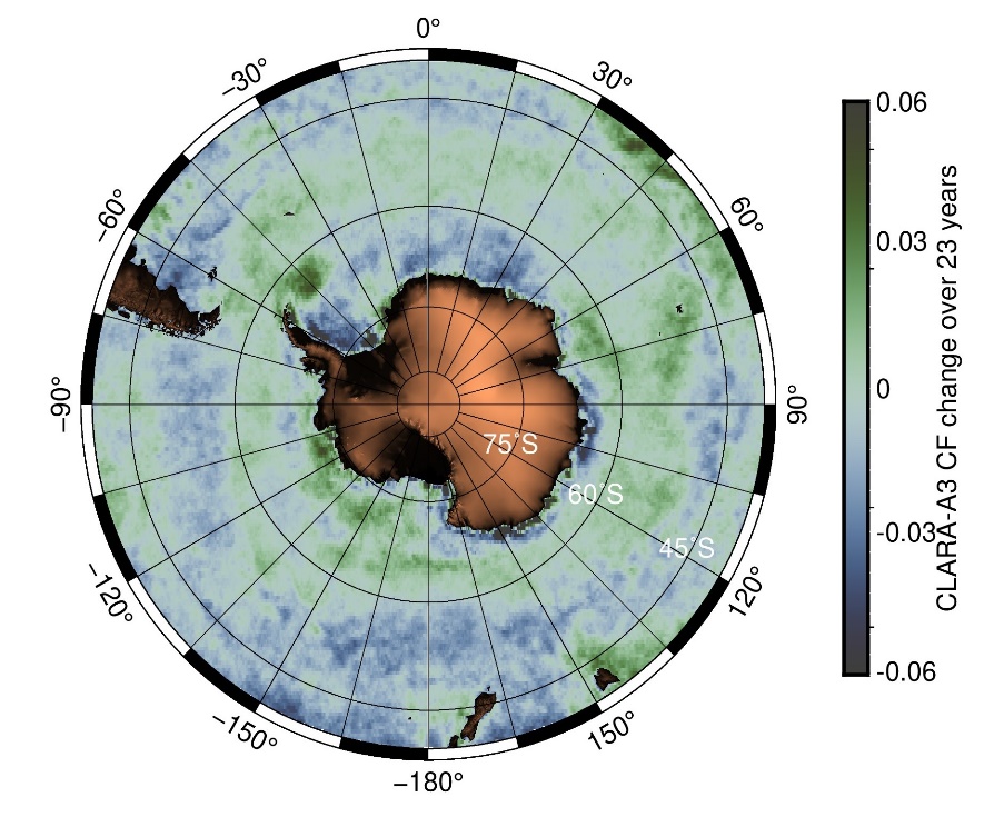
Figure S1: Annual rates of change in photosynthetically available radiation (PAR) and cloud fraction (CF). (A) PAR trend from Globcolour data over the 1998 to 2021 time frame. Contours represent the mean positions of frontal regions from north to south: red - Northern Boundary (NB), orange - Subantarctic Front (SAF), yellow - Polar Front (PF), green - Southern Antarctic Circumpolar Current Front (SACCF), and blue - Southern Boundary (SB). (B) Cloud fraction trend derived from Coperncius CLARA-A3 (S1B) over 1998 to 2020.
Table S1. Number of observations (n) used to calculate monthly mean chlorophyll-a concentrations for each frontal region and the Southern Ocean.
| Month | 40°S–NB | NB–SAF | SAF–PF | PF–SACCF | SACCF–SB | SB–AntCoastline | Southern Ocean |
|---|---|---|---|---|---|---|---|
| Jan | 26 | 26 | 26 | 26 | 26 | 26 | 26 |
| Feb | 26 | 26 | 26 | 26 | 26 | 26 | 26 |
| Mar | 26 | 26 | 26 | 26 | 26 | 26 | 26 |
| Apr | 26 | 26 | 26 | 26 | 26 | 16 | 26 |
| May | 26 | 26 | 26 | 26 | 9 | 0 | 18 |
| Jun | 26 | 26 | 26 | 1 | 0 | 0 | 0 |
| Jul | 26 | 26 | 26 | 19 | 0 | 0 | 2 |
| Aug | 26 | 26 | 26 | 26 | 26 | 0 | 26 |
| Sep | 26 | 26 | 26 | 26 | 26 | 0 | 26 |
| Oct | 26 | 26 | 26 | 26 | 26 | 0 | 26 |
| Nov | 26 | 26 | 26 | 26 | 26 | 8 | 26 |
| Dec | 26 | 26 | 26 | 26 | 26 | 26 | 26 |
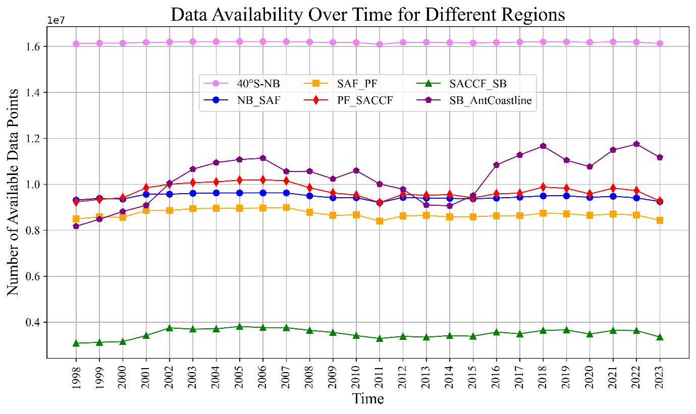
Figure S2: 1998–2023 time series of annual total number of available data points in the Copernicus-GlobColour data set.
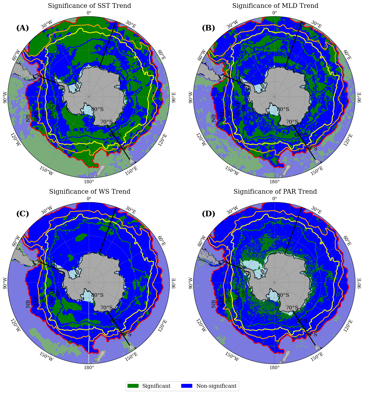
Figure S3. Significance maps for the trends of of sea-surface temperature (SST), mixed-layer depth (MLD), wind speed (WS) and photosynthetically available radiation (PAR) displayed in Figure 2.7.
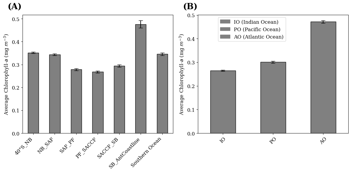
Figure S4: Average Chl-a concentrations per frontal regions and sectors of the SO from the ESA OC-CCI data (1998-2023). 26-year average Chl-a values (mg m-3) \[mean, SE\] within (A) each frontal region and the entire SO, where NB= northern boundary, SAF= Sub Antarctic Front, PF=Polar Front, SACCF= Southern ACC Front, SB= Southern boundary, and (B) the Indian, Pacific and Atlantic Sectors of the SO.
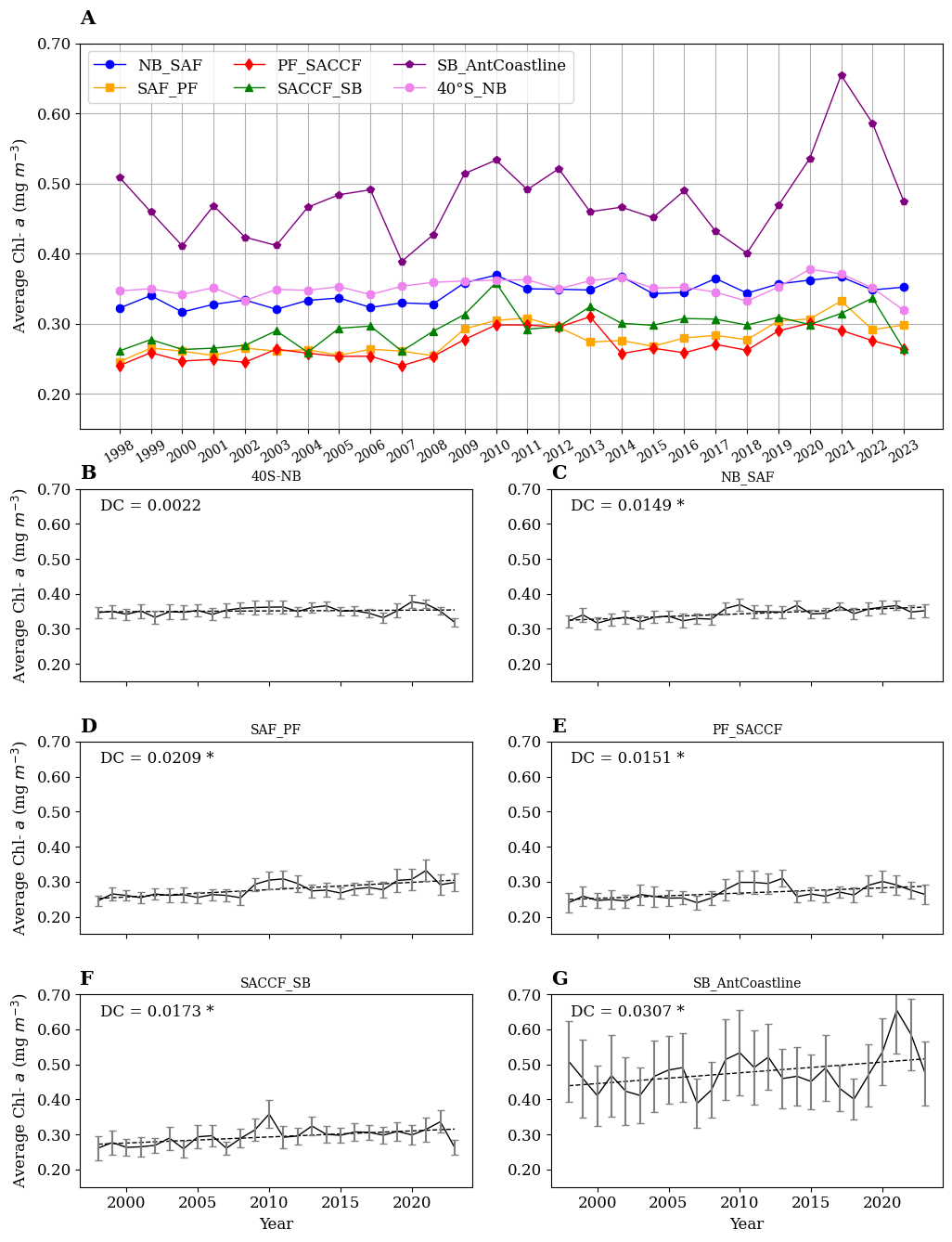
Figure S5: Annual average surface Chl-a (mg m-3) from 1998 to 2023 in the SO and the six frontal regions (A). For clarity, the six frontal regions, as indicated (B to G) are shown separately with their standard error, based on the ESA OC-CCI merged ocean colour product. The dashed lines are the linear trends, and the "DC" values indicated in each panel are the decadal Chl-a changes, in mg Chl-a m-3). The asterisks (*) denote significance level at 95% confidence.
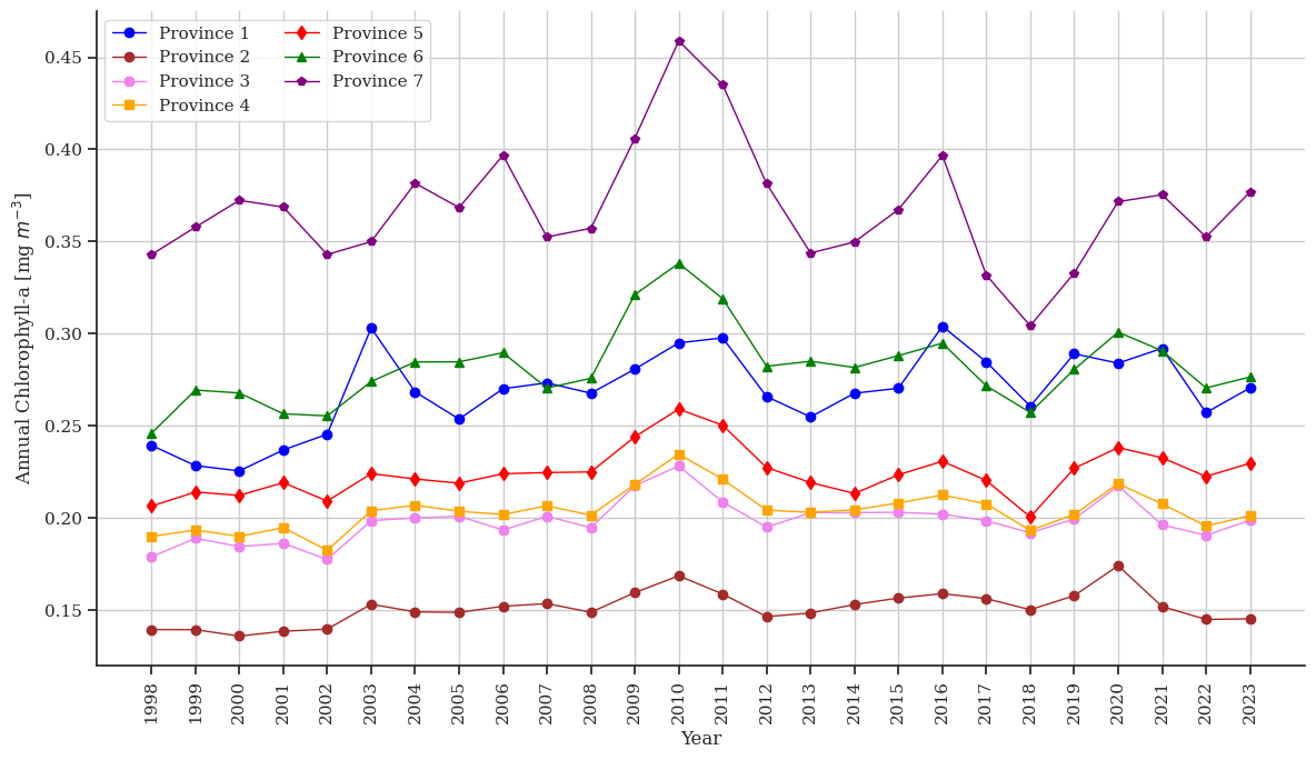
Figure S6: 1998–2023 time series of annual average surface Chl-a for the Ardyna’s provinces.
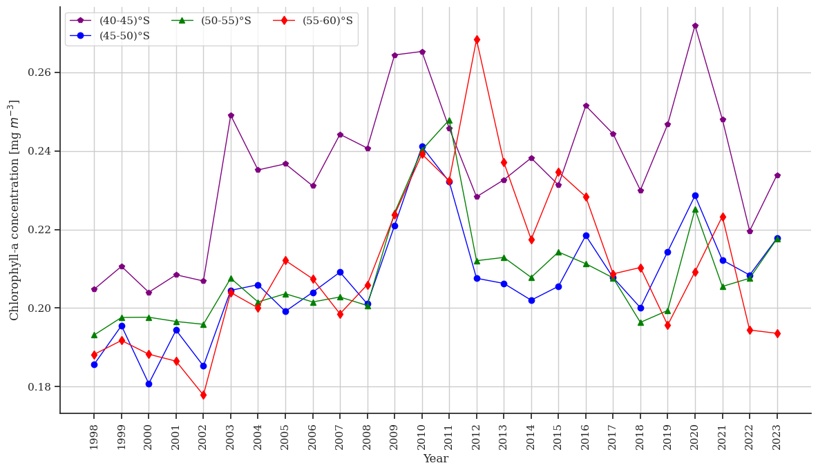
Figure S7: 1998–2023 time series of annual average surface Chl-a for fixed latitudinal bands.
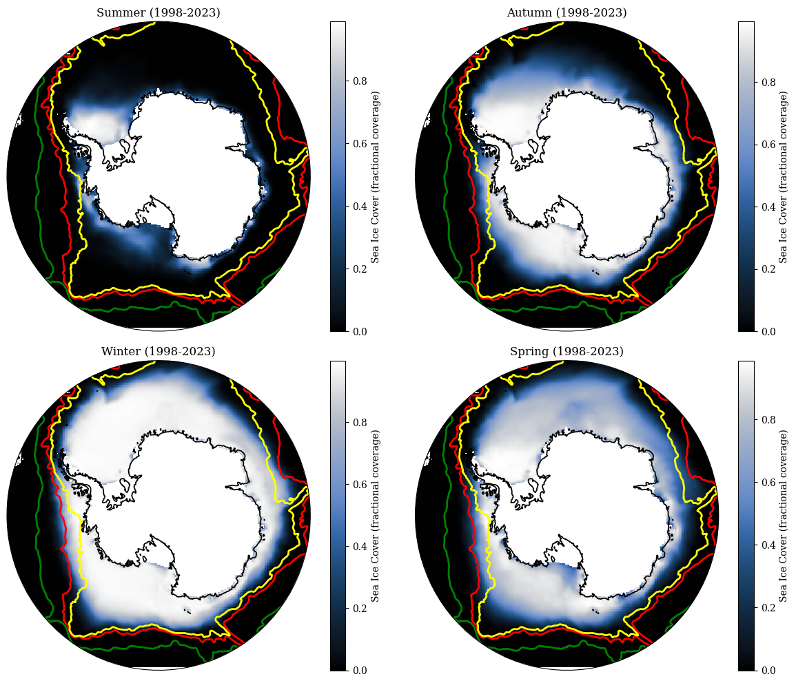
Figure S8: Seasonal composite of sea ice coverage in the Southern Ocean. The yellow line indicates the Southern Boundary (SB) front, the red line in the Southern Australian Circumpolar Current (ACC) Front (SACCF) and the green line the Polar front (PF).
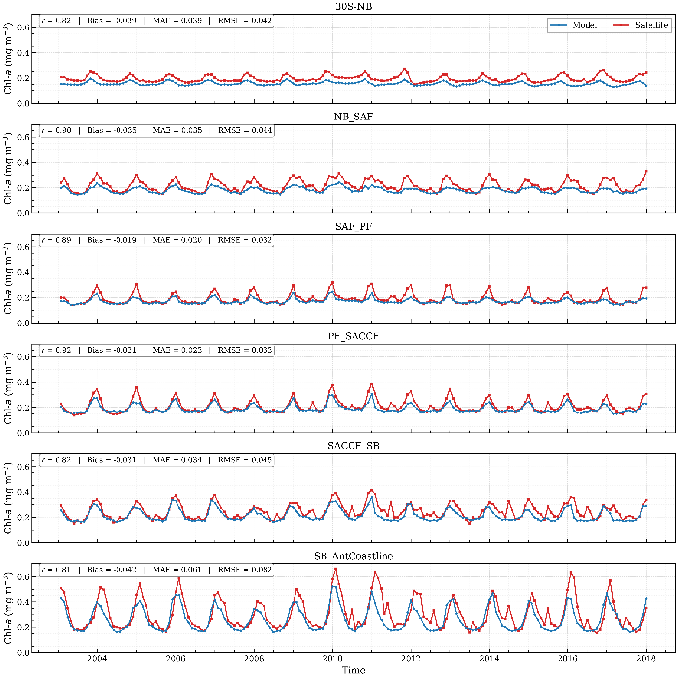
Figure S9: Time-series comparison of satellite-observed and U-Net-reconstructed chlorophyll a (Chl-a) across Southern Ocean frontal zones from 2003 to 2017. Satellite Chl-a is shown in blue, while reconstructed Chl-a is shown in red.