2 Physical Drivers of Long-term Chlorophyll-a Variability in the Southern Ocean
This chapter is an edited version of a paper that has been published as Golder, M. R., & Antoine, D. (2025). Physical drivers of long-term chlorophyll-a variability in the Southern Ocean. Elem Sci Anth, 13(1), 00077. DOI: 10.1525/elementa.2024.00077.
2.1 Abstract
Despite the critical roles of the Southern Ocean in marine biodiversity and the global carbon cycle, there is a significant gap in understanding how physical drivers shape the long-term variability of phytoplankton at the base of this extensive marine ecosystem and the carbon it exports. Here we used monthly satellite ocean colour observations to assess seasonal and interannual variability and long-term trends of phytoplankton in the Southern Ocean. Over the 26 years we studied (1998–2023), seasonal variations in the concentration of chlorophyll-a (Chl-a, a proxy for phytoplankton biomass) were statistically significant, with the highest values (mean ± standard error of 0.305 ± 0.001 mg m–3, n = 78) in summer (January–March) and lowest (0.169 ± 0.003 mg m–3, n = 54) in winter (July–September). The highest and lowest annual Chl-a values across the entire Southern Ocean were observed in 2010 and 2018, respectively. A 5-to-6-year cycle was also observed for areas south of the Polar Front. Over the 26 years, 60% of the Southern Ocean showed an increase in Chl-a. We then assessed the concurrent changes in Chl-a and four potential environmental variables of its variability, namely the sea surface temperature, mixed-layer depth, wind speed and above-surface photosynthetically available radiation. This analysis revealed complex patterns of either parallel or opposite changes in Chl-a and these four physical variables When annual anomalies (de-seasonalised data) of Chl-a were regressed against anomalies of the physical variables, sea surface temperature and photosynthetically available radiation showed stronger correlations with Chl-a than did mixed-layer depth and wind speed in about 75% of the Southern Ocean. Further investigation incorporating additional variables, such as large-scale climate drivers and sea ice variability, is needed to achieve a clearer understanding of multi-decadal phytoplankton variability in the Southern Ocean.
2.2 Introduction
In an era of rapid global environmental change, the Southern Ocean has emerged as a critical barometer for ecological responses to the changes involved, revealing in particular their possible impacts on phytoplankton biomass and community composition. This study delves into the long-term spatiotemporal decadal variability of phytoplankton in the Southern Ocean by using 26 years of satellite ocean colour data. We sought to unravel the intricate relationships between phytoplankton and the physical variables of sea surface temperature (SST), photosynthetically active radiation (PAR), mixed-layer depth (MLD), and wind speed (WS).
The Southern Ocean, encompassing the waters south of the Subtropical Front, is a vast and dynamic system that plays a critical role in Earth's climate and carbon cycles. As the largest basin for anthropogenic CO2 and a key modulator of heat distribution, the Southern Ocean influence extends far beyond its geographical boundaries (Canadell et al., 2023; Hauck et al., 2023; Morrison et al., 2022). Phytoplankton communities are the foundation of the Southern Ocean ecosystem, driving the biological carbon pump through photosynthetic carbon fixation (Hauck et al., 2018). The Southern Ocean also serves as a conduit between the surface and the deep ocean (Canadell et al., 2021, 2023). Modelling studies suggest that it absorbs approximately 50% of the total global-ocean uptake of anthropogenic CO2 (DeVries et al., 2017) and 75% of the excess heat from human activities (Frolicher et al., 2015). The CO2 exchange is driven by physical mechanisms and modulated by biological activity. CO2 outgassing occurs in winter due to mixing and upwelling of deep waters. In contrast, during summer, the peak activity of phytoplankton and carbon export to the deep ocean enhances CO2 uptake, emphasizing the dominant role of the biological carbon pump (Hauck et al., 2018; Thomalla et al., 2023).
Phytoplankton growth in the Southern Ocean is driven by light (PAR) and nutrient availability, and influenced by other various environmental variables such as SST (Deppeler & Davidson, 2017; Petrou et al., 2016). Models indicate that the ongoing rise in atmospheric CO2, which under some scenarios of climate change is projected to reach 750 µatm by 2100, will induce a myriad of changes in the Southern Ocean, including altered nutrient input patterns, increased vertical mixing, upper-ocean warming, and ocean acidification (Henley et al., 2020; Pörtner et al., 2019). Some of these changes are expected to affect the MLD, thereby controlling nutrient and light availability to phytoplankton, which is crucial for their growth (Carranza & Gille, 2015). The impact of climate change on the Southern Ocean already manifests in the southward migration of ocean fronts, variations in SST, and alterations in sea ice coverage (Constable et al., 2014; Deppeler & Davidson, 2017). Such transformations control the phytoplankton habitats by influencing nutrient and light availability (Arrigo et al., 2008; Boyd et al., 2008), altering the duration of phytoplankton growth seasons, and impacting the phenology of the community, thereby reshaping phytoplankton dynamics and the broader biogeochemical cycles (Joy-Warren, 2022).
Therefore, the future of phytoplankton in the Southern Ocean under rising CO2 concentrations and global warming is uncertain. Various factors, such as changes in MLD, PAR and wind-driven mixing of nutrients, as well as temperature, salinity, atmospheric deposition, and climate change, could lead to divergent outcomes for primary productivity and the associated export production (Boyd, 2019). For example, decreased wind stress can reduce the upward transport of nutrients. Changes in MLD can affect nutrient availability and light exposure for phytoplankton, while variations in incoming PAR directly drive the rate of photosynthesis and overall productivity (Hopkins et al., 2021).
These environmental variables all potentially influence the concentration and distribution of phytoplankton in the Southern Ocean. Temperature impacts the dark reactions of photosynthesis and consequently affects phytoplankton growth. PAR drives photosynthesis. While MLD deepening brings nutrients to the surface, promoting phytoplankton growth, it can also carry phytoplankton to depths where light is limiting photosynthesis. WS promotes vertical mixing, which further affects nutrient transport and MLD, thereby influencing phytoplankton distribution patterns in the Southern Ocean (Carranza & Gille, 2015). In addition to these bottom-up drivers, top-down control through grazing by zooplankton also controls phytoplankton biomass in the Southern Ocean. Studies indicate that zooplankton grazing significantly reduces phytoplankton standing stock, often explaining the low chlorophyll levels observed in Antarctic waters (Knox, 2007; Minas & Minas, 1992).
Over the past 15 years, a concerted effort has been made to monitor and understand the changes in global ocean phytoplankton densities (Martinez, Gorgues, et al., 2020; Mishra et al., 2022; Zhai et al., 2024). These endeavours have spanned from experimental studies to sophisticated observational techniques, aiming to appraise the present condition and forecast future trajectories of phytoplankton. Notably, larger cell phytoplankton (mainly diatoms) dominated during 2002–2015 in the Southern and Arctic Oceans, while coccolithophores prevailed elsewhere (Mishra et al., 2022). In addition, Van Oostende et al. (2023) analyzed ocean colour trends globally, observing increased concentrations of chlorophyll-a (Chl-a) in polar waters and decreased concentrations in some equatorial regions. However, the broader body of these studies was limited to the low-to-medium latitude oceans (50°N–50°S).
Despite its critical role in the Earth's climate and ocean productivity, the Southern Ocean remains relatively under-studied, primarily due to its remoteness and the challenging conditions that hinder extensive field research (Joy-Warren, 2022). A handful of studies have been undertaken to interpret phytoplankton trends and primary productivity in the Southern Ocean using remote sensing data. Notably, Del Castillo et al. (2019) and Pinkerton et al. (2021) observed a rise in chlorophyll concentrations using the dataset from 1999 to 2018, while Prend et al. (2022) noted that the year-to-year fluctuations in annual mean chlorophyll were only weakly tied to the Southern Annular Mode. Ardyna et al. (2017) suggested that local advective currents and iron supply processes predominantly influenced regional phytoplankton biomass. These studies, while shedding light on trends of Chl-a, leave us uncertain about what might happen in the future. They also fall short in linking these biological changes to other environmental drivers, leaving a significant gap in our comprehension of the response of phytoplankton communities to environmental shifts. The underlying mechanisms of the decadal variability of the Southern Ocean phytoplankton remain insufficiently understood (Canadell et al., 2023; Gruber et al., 2019; Hauck et al., 2020; McKinley et al., 2020).
Long-term, consistent observations over broad spatiotemporal scales are essential to improve this understanding, and satellite remote sensing and autonomous platforms offer such data (Ardyna et al., 2017; Arrigo et al., 2008; Briggs et al., 2018; Claustre et al., 2020; Del Castillo et al., 2019; Prend et al., 2022). Satellite ocean colour is the main tool for global, high-temporal-resolution ocean ecosystem observations (Martinez, Gorgues, et al., 2020; Mishra et al., 2022; Zhai et al., 2024). However, certain features, such as deep chlorophyll maxima and algal blooms beneath sea ice, cannot be measured using this approach. Therefore, this study only deals with the average surface chlorophyll in the first optical depth. This depth is about 20 m for the clearest waters of the Southern Ocean (Chl-a of approximately 0.1 mg m–3), which does not exceed the mixed layer depth in most instances. Therefore, we took the satellite-derived Chl-a to be representative of the average Chl-a over the entire mixed layer. We used satellite-derived Chl-a from the satellite ocean colour time series available to date, i.e., from 1998 to 2023, to assess phytoplankton changes in the Southern Ocean and analyze their connections to four potential physical drivers (SST, MLD, PAR, and WS). Given the physical and biological dynamics at ocean fronts in the Southern Ocean (Arrigo et al., 2008; Chapman et al., 2020; Palter et al., 2013), we focused most of our analyses on regions defined by these fronts.
2.3 Data and Methods
2.3.1 The Southern Ocean and its frontal regions
Here, we define the Southern Ocean as all waters south of the long-term average position of the Subtropical Front, which we refer to as the northern boundary (NB; Figure 2.1) following Park and Durand (2019). The Southern Ocean is subdivided by four other fronts, namely (from south to north), the Southern Boundary Front (SB), the Southern Antarctic Circumpolar Current Front (SACCF), the Polar Front (PF), and the Subantarctic Front (SAF). The average positions of these fronts are taken from Park and Durand (2019); Park et al. (2019), who derived them from the mean ocean dynamic topography calculated using satellite altimetry data.
In our analysis of long-term changes in Chl-a, we used fixed frontal positions to provide a consistent spatial reference across years. While we acknowledge that oceanographic fronts can shift over time, this approach enables tracking inter-frontal variability without conflating spatial shifts in frontal positions with temporal changes in water properties. We recognize that some overlap is inevitable; however, using fixed boundaries allows for systematic comparison over the 26-year period.
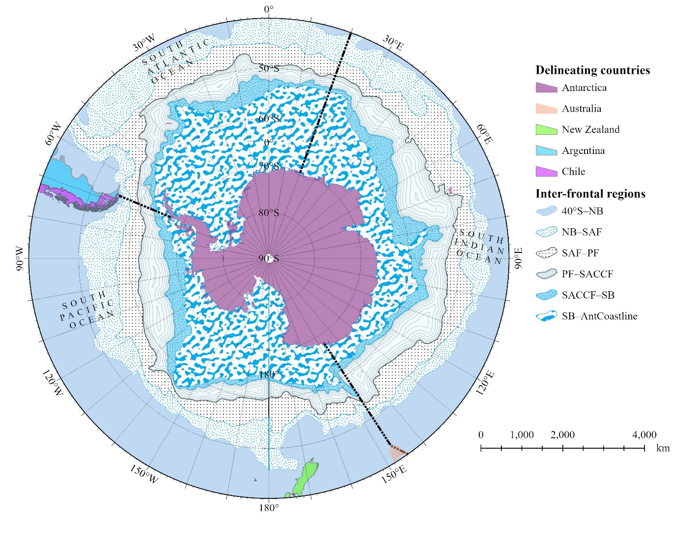
Figure 2.1:Study regions in the Southern Ocean: boundaries and inter-frontal regions. Map showing the inter-frontal study regions in the Southern Ocean bounded from north to south by the 40°S latitudinal band, the Northern Boundary (NB), Subantarctic Front (SAF), Polar Front (PF), Southern Antarctic Circumpolar Current Front (SACCF), Southern Boundary (SB), and the Antarctic coastline (AntCoastline). The Atlantic, Indian, and Pacific sectors of the Southern Ocean, also considered in this study, are separated by dotted black lines.
This distinction is important because analyzing long-term changes using fixed latitude bands across the entire Southern Ocean could introduce confusion between spatial and temporal variability. For example, the latitudinal band between 55°S and 60°S spans parts of all inter-frontal regions in the Southern Ocean, except between the NB and SAF (NB_SAF in Figure 2.1), when considering the entire circumpolar region. Monthly data for an inter-frontal region were included only if at least 40% of its area had data available for that month.
In using fixed frontal boundaries, we assumed that the same water masses were followed over time within the region between two fronts. This approach allowed us to focus on inherent changes within these water masses, irrespective of their possible long-term spatial movement. Although frontal positions can vary on monthly and annual time scales, we assumed that these changes were limited enough over the 26 years examined that we could use average, fixed positions for these fronts. This choice is supported by the results of several studies (Gille, 2014; Graham et al., 2012; Shao et al., 2015), which did not find significant changes of the positions of these fronts over the past 2 decades. Sensitivity analyses related to this choice are discussed later.
Accordingly, the study region was subdivided into six inter-frontal zones, defined by their frontal boundaries: region 1, from 40ºS to the NB (40°S–NB); region 2, from the NB to the SAF (NB–SAF); region 3, from the SAF to the PF (SAF–PF); region 4, from the PF to the SACCF (PF–SACCF); region 5, from the SACCF front to the SB (SACCF–SB); and region 6, from the SB to the Antarctic coastline (SB–AntCoastline; Figure 2.1). The 40°S–NB area was included as a boundary to the Southern Ocean, which ends at the nominal NB; results are displayed and discussed primarily for the other five regions. The relative areas of these zones vary substantially, with SB–AntCoastline being the largest (45.5% of the total Southern Ocean area) and SACCF–SB the smallest (7.9%; Table 2.1).
|
|
|
|---|---|---|
|
|
|
|
|
|
|
|
|
|
|
|
|
|
|
|
|
|
|
|
|
aNorthern Boundary (NB), Subantarctic Front (SAF), Polar Front (PF), Southern Antarctic Circumpolar Current Front (SACCF), Southern Boundary (SB), and Antarctic coastline (AntCoastline).
Although the distribution of physical and biogeochemical properties in the Southern Ocean is largely driven by the latitudinal arrangement of fronts, this ocean also shows distinct average properties within its Indian (30°E–150°E), Pacific (150°E–60°W), and Atlantic (60°W–30°E) sectors (Turner et al., 2009). Therefore, results are also presented according to these sectors.
2.3.2 Datasets
We used satellite-derived Chl-a concentrations from the Copernicus Marine Environment Monitoring Service (CMEMS) multi-mission merged ocean colour data set, named GlobColour (CMEMS, 2023a; Garnesson et al., 2019). This data set is built from observations by the US National Oceanic and Atmospheric Administration Visible Infrared Imaging Radiometer Suite (VIIRS), the US National Aeronautics and Space Administration (NASA) Moderate Resolution Imaging Spectroradiometer (MODIS), the European Space Agency (ESA) Medium Resolution Imaging Spectrometer (MERIS), and the NASA Sea-viewing Wide Field-of-View Sensor (SeaWiFS). It comes as daily non-interpolated Level 3 Mapped 4 × 4 km resolution products encompassing 26 years from January 1998 to December 2023, which we then averaged into monthly data (Table 2.2). Using this merged data product overcomes the limitations of single satellite datasets and allows a comprehensive insight into the decade-long dynamics of phytoplankton in the Southern Ocean. In this study, we defined the seasonal periods as summer (January, February, March), autumn (April, May, June), winter (July, August, September), and spring (October, November, December).
A sensitivity analysis was also carried out by using the ESA Ocean Colour Climate Change Initiative (OC-CCI) data set (Sathyendranath et al., 2021) instead of the Copernicus GlobColour data set. To ensure that only open-water conditions were analysed, Chl-a data points coinciding with non-zero sea ice concentration (SIC > 0) were excluded based on sea ice concentration data from the US National Snow and Ice Data Center (NSIDC).
For SST, we used data from the UK Met Office derived through the Operational SST and Sea Ice Analysis (OSTIA) system, accessible from CMEMS (Good et al., 2020). This product, published by the Group for High-Resolution Sea Surface Temperature (GHRSST) includes daily SST data from October 1, 1981, presented on a regular global grid with a resolution of 0.05° (Brasnett, 2008). The level 4 product integrates satellite-derived infrared and microwave data with in-situ observations, producing a detailed, high-resolution output (Ferster et al., 2018). To align the SST data with the ocean colour dataset, we computed the monthly average of daily SST data from January 1998 to December 2023 (Table 2.2).
For MLD, we used the Multi Observation Global Ocean 3D Temperature Salinity Height Geostrophic Current and MLD data set, which comes at a spatial resolution of 0.25° (CMEMS, 2023b) and also covers the time window from January 1998 to December 2023 (Table 2.2). This dataset is derived from a combination of in-situ and satellite observations. The MLD was calculated as the minimum depth of two MLD values determined by density and temperature criteria (de Boyer Montégut et al., 2004). The temperature criterion determined MLD as the depth where temperature was lower than the value at 10 m by 0.2°C, and the density criterion determined MLD as the depth where density was larger than the value at 10 m by a density difference which corresponded to a local temperature decrease by 0.2°C. For a detailed description of the dataset and processing methods, see Guinehut et al. (2012). Utilizing density and temperature criteria prevents potential overestimation or underestimation, providing a more accurate determination of the MLD at high latitudes (Guinehut et al., 2012).
Monthly WS data were taken from the merged Cross-Calibrated Multi-Platform (CCMP) wind vector analysis product created by Remote Sensing Systems (RSS). This CCMP reanalysis product combines wind vector data from various sources, including moored buoys and satellite scatterometers, offering enhanced reliability at high frequencies compared to individual scatterometers (Atlas et al., 2011). Additionally, compared to other wind products, it shows stronger relationships with MLD (Atlas et al., 2011; Carranza & Gille, 2015). The integrated wind dataset is accessible on the RSS website (Mears et al., 2022) with a spatial resolution of 25 km (Table 2.2).
As for PAR (Einsteins m−2 day−1), we used monthly data which are based on (Frouin et al., 2003). This dataset is presented on the same 4-km resolution grid as the Chl-a products (Table 2.2). We initially tested the GlobColour PAR product for consistency with the use of the GlobColour Chl-a. This product, however, showed a significant and quasi-ubiquitous 26-year decrease over the Southern Ocean, which we considered unrealistic and was indeed inconsistent with the cloudiness trend that we derived from independent cloud data (Figure S1).
| Variablea | Temporal resolution | Spatial resolution | Projectb | Sourcec | Monitoring period |
|---|---|---|---|---|---|
| Chl-a | Daily | 4 km | Globcolour | CMEMS | 1998–2023 |
| SST | Daily | 0.05° | GHRSST | CMEMS | 1998–2023 |
| MLD | Monthly | 0.25° | N/A | CMEMS | 1998–2023 |
| WS | Monthly | 0.25° | N/A | RSS | 1998–2023 |
| PAR | Monthly | 4 km | MODIS | OB:DAAC | 2003–2023 |
aChlorophyll-a (Chl-a), sea surface temperature (SST), mixed layer depth (MLD), wind speed (WS), and photosynthetically available radiation (PAR)
bCopernicus Globcolour, Group for High-Resolution Sea Surface Temperature (GHRSST), and Moderate Resolution Imaging Spectroradiometer (MODIS)
eCopernicus Marine Environment Monitoring Service (CMEMS), Remote Sensing Systems (RSS), and Ocean Biology: Distributed Active Archive Center (OB:DAAC)
In this study, we quantified linear trends in Chl-a, SST, MLD, WS, and PAR for the entire Southern Ocean and for inter-frontal zones and ocean sectors by calculating the Sen slope (Sen, 1968) from monthly anomaly data. The anomalies were calculated by subtracting the monthly climatology from the corresponding monthly values, effectively removing seasonality and addressing non-normality in the raw data. The Sen slope, which estimates the median of all slopes between all pairs of points in the time series, was chosen due to its robustness against outliers (Hipel & McLeod, 1994). The statistical significance of the detected trends was assessed using the non-parametric Mann-Kendall test, which does not require the assumption of normality (Kendall, 1948; Mann, 1945). To account for autocorrelation in the time series, we applied the correction method proposed by (Yue & Wang, 2004). A trend was considered statistically significant if it exceeded the 95% confidence level (i.e., p < 0.05) based on a t-test. To further the comparative and qualitative analysis of the trends in Chl-a and its potential drivers (SST, MLD, PAR, WS), we calculated the slope and regression coefficient of the relationship between their monthly anomalies to avoid that the relationship be driven by the seasonal cycles. These anomalies were calculated by removing the 26-year monthly average values from the data in each month, which is de-seasonalizing the data.
2.3.3 Sensitivity test
We conducted several sensitivity analyses to assess the robustness of our results. We focused on: 1) which data source was used for Chl-a, 2) the choice of calculating average values over inter-frontal regions, and 3) the varying sea ice coverage for the seasonal sea ice zone (SB–AntCoastline region).
To the best of our knowledge, there are only two global multi-sensor ocean colour merged data sets that could have been used for this study: the Copernicus GlobColour multi-mission merged data set (CMEMS, 2023a) and the ESA OC-CCI data set. We selected the former because the latter is generated through the Polymer algorithm (Steinmetz et al., 2011). This algorithm couples an ocean bio-optical model (Morel & Maritorena, 2001) and a simplified atmospheric model to iteratively derive the best solution for the remote-sensing reflectance and the parameters of the atmospheric model. This technique has proven efficient in processing satellite ocean colour observations, in particular in sub-optimal conditions where many algorithms would fail (e.g., thin clouds or moderate sun glint). We considered, however, that the constraint imposed by the built-in bio-optical model might make generating a data set for analysis of long-term trends inappropriate. Indeed, Polymer will always lean towards a solution that pushes the remote-sensing reflectance (Rrs) spectra to fit the bio-optical model embedded within it. This pushing carries some risk of biasing long-term changes in Rrs in the case of actual bio-optical relationships changing significantly over time. We performed the sensitivity analyses by generating the entire set of results derived from the GlobColour data set from the ESA OC-CCI data set as well.
We analyzed data within inter-front regions assuming that this approach would minimize the risk of merging data from different oceanographic water masses compared to using fixed latitude bands, which could generate spurious temporal trends. To illustrate the impact of changing the way of calculating average values across the Southern Ocean, we repeated the analysis of Chl-a values using fixed latitude bands of 5 degrees each, starting at 40°S. We also used the seven provinces defined by Ardyna et al. (2017) as regions to follow with time.
Because satellite ocean colour data are only available when there are ice-free waters and sunlight, the seasonal sea ice zone (included in the SB–AntCoastline region) could have varying annual coverage, affecting Chl-a averages. To assess the potential impact of this variability, we generated a gap-free 26-year average Chl-a map by combining any data from ice-free areas within the SB–AntCoastline region. We then calculated average annual Chl-a values for each year by excluding areas covered by sea ice, using monthly sea ice coverage data from the NSIDC (DiGirolamo et al., 2022).
2.4 Results
2.4.1 General traits of spatial and seasonal variability of phytoplankton in the Southern Ocean
The spatial variability of Chl-a in the Southern Ocean is illustrated in Figure 2.2A, which displays the 26-year average concentration (January 1998 to December 2023). For high latitudes, the average can be calculated only for summer months when sunlight allows observations by satellite ocean colour above ice-free waters. The highest Chl-a concentrations (above approximately 0.45 mg m–3) are observed from the SB to the Antarctic coast, particularly in the Ross Sea and Western Antarctic Peninsula regions (dark blue rectangular box in Figure 2.2A). Conversely, Chl-a concentrations below about 0.2 mg m–3 are observed in most other areas, except along the northern boundary in the Atlantic sector and east of Africa. The coefficient of variation of Chl-a (Figure 2.2B) is high (CV > 80%) south of the SB in the seasonal ice zone, around the Kerguelen plateau and Heard Island, and on the Patagonian shelf. Other areas, e.g., the SAF and PF regions in the Pacific and Indian sectors have lower variability.
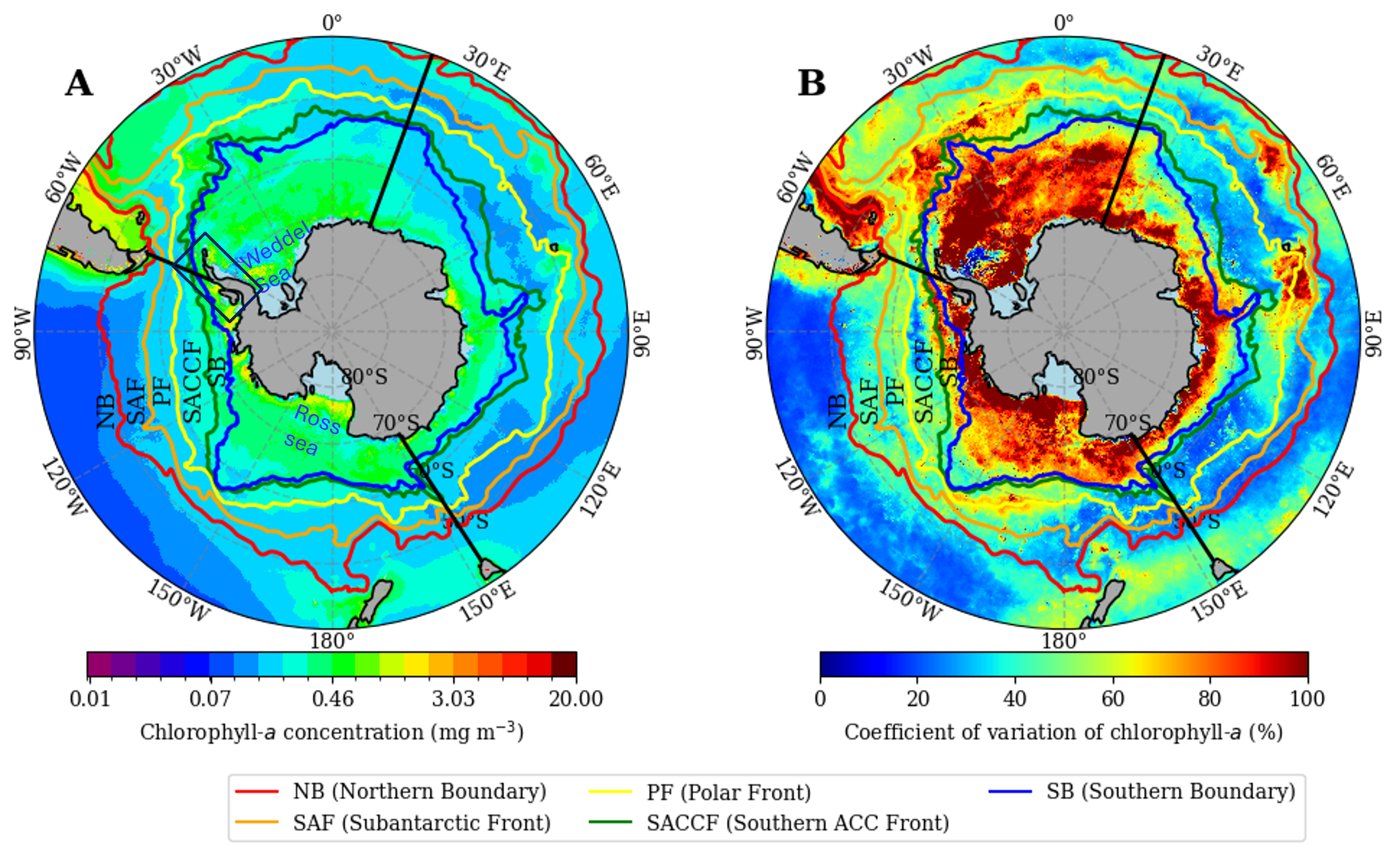
Figure 2.2: Maps of mean chlorophyll-a concentration and its coefficient of variation. A) 26-year average of the Copernicus Globcolour (1998–2023) surface chlorophyll-a concentration (mg m–3). B) Coefficient of variation of surface chlorophyll-a (%). Color-coded lines indicate the mean positions of the fronts; ACC indicates Antarctic Circumpolar Current.
The average Chl-a values within the six inter-frontal regions are shown in Figure 2.3A. The highest average value was found in the region between the SB and Antarctic coastline (mean ± standard error, SE, of 0.41 ± 0.01 mg m–3, range of 0.20–0.70 mg m–3, n = 128) and the lowest between the SAF and PF (0.19 ± 0.003 mg m–3, range of 0.13–0.40 mg m–3, n = 312). Statistically significant differences (χ2(df = 6) = 487.38, p < 0.05, Kruskal-Wallis H test) were observed across all frontal zones, indicating that the mean Chl-a values vary significantly between regions. Post hoc comparisons further revealed that PF–SACCF, SAF–PF, and SB–AntCoastline differed notably from the Southern Ocean. Significant (p < 0.05) regional differences in mean Chl-a concentration were also observed by sector, as shown in Figure 2.3B, with the highest mean in the Atlantic sector (0.32 ± 0.07 mg m–3, range of 0.22–0.51 mg m–3, n = 312), followed by the Pacific sector (0.19 ± 0.04 mg m–3, range of 0.13–0.35 mg m–3, n = 312) and the Indian sector (0.18 ± 0.03 mg m–3, range of 0.14 to 0.28 mg m–3, n = 312; Figure 2.3B).
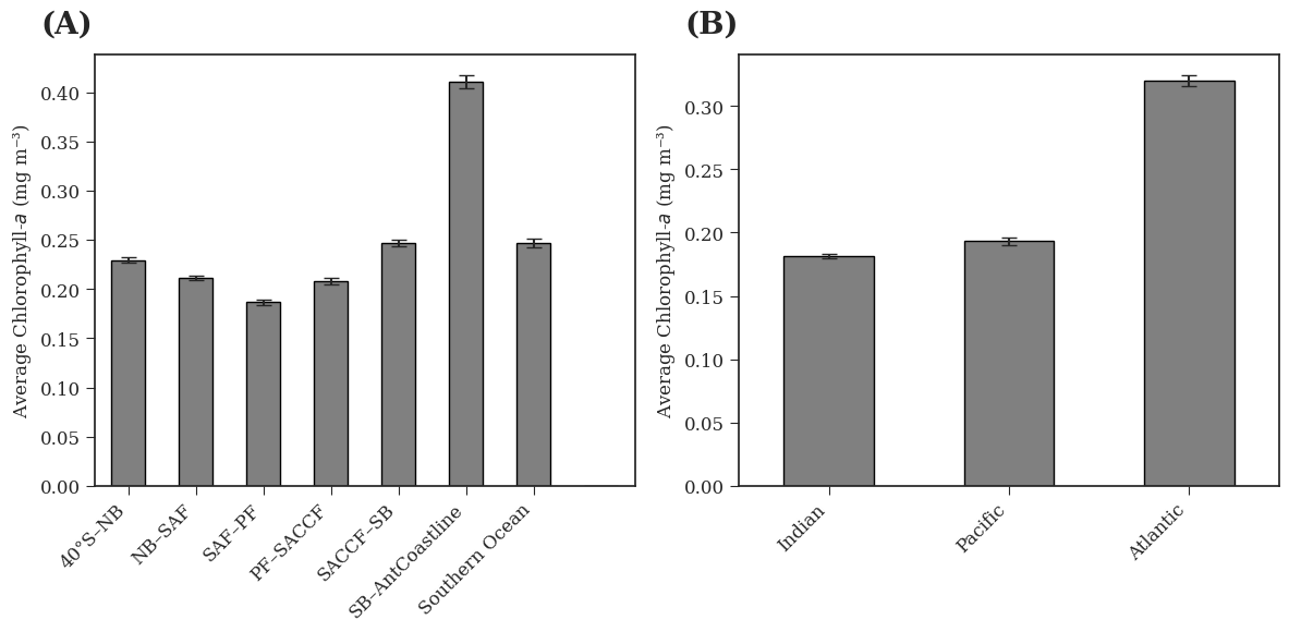
Figure 2.3: Mean chlorophyll-a concentrations in inter-frontal regions and sectors of the Southern Ocean. A) The 26-year (1998–2023) average chlorophyll-a concentration (mg m–3) within each inter-frontal region and the entire Southern Ocean, where the regions are defined, and ordered north to south, by the Northern Boundary (NB), Subantarctic Front (SAF), Polar Front (PF), Southern Antarctic Circumpolar Current Front (SACCF), Southern Boundary (SB), and Antarctic coastline (AntCoastline). Error bars indicate standard error (SE), where n ranges from 128 to 312. B) Average chlorophyll-a concentration (mg m–3) in the Indian, Pacific and Atlantic sectors of the Southern Ocean. Error bars indicate SE, where n = 312. Data were included only if at least 40% of the area had valid observations for a given month. Based on this threshold, no data were available for SB–AntCoastline from May to October or for SACCF–SB in June and July.
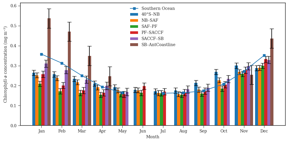
Changes in the 26-year average monthly Chl-a concentrations followed a consistent seasonal pattern for the five inter-frontal regions of the Southern Ocean (Figure 2.4), with maxima of 0.30–0.54 mg m–3 from November to March and rather steady low values (below approximately 0.2 mg m–3) from May to September (significant seasonal differences at p < 0.05). The highest monthly average Chl-a concentration of 0.54 mg m–3 (range of 0.40–0.70 mg m–3) was recorded in January in the SB–AntCoastline region, and the lowest monthly average of 0.16 mg m–3 (range of 0.14–0.17 mg m–3) was recorded in August in the region between SAF and PF (Figure 2.4). The seasonal (3-month) variations in Chl-a concentrations across different regions of the Southern Ocean are provided in Table 2.3. During spring (October–December), Chl-a concentrations were generally higher compared to the other seasons in a given region. For instance, in the SAF–PF region, the spring Chl-a concentration averaged 0.245 mg m–3, while the lowest mean concentration was observed in autumn (0.169 mg m–3). For the entire Southern Ocean, however, the highest mean Chl-a concentration was observed in summer (January–March) In the SB–AntCoastline region, for example, the highest Chl-a concentration was observed in summer (0.452 ± 0.012 mg m–3), and the lowest in autumn (0.191 ± 0.004 mg m–3), noting that winter (July–September) had no data for this region (Table 2.3).
| Regions | Summer (Jan–Mar) | Autumn (Apr–Jun) | Winter (Jul–Sep) | Spring (Oct–Dec) | Annual range (Max – Min) |
|---|---|---|---|---|---|
| 40°S–NB | 0.244 ± 0.004 (n=78) | 0.188 ± 0.002 (n=78) | 0.181 ± 0.003 (n=78) | 0.279 ± 0.004 (n=78) | 0.07 |
| NB –SAF | 0.236 ± 0.003 (n=78) | 0.182 ± 0.002 (n=78) | 0.167 ± 0.002 (n=78) | 0.262 ± 0.004 (n=78) | 0.06 |
| SAF –PF | 0.182 ± 0.003 (n=78) | 0.158 ± 0.002 (n=78) | 0.159 ± 0.001 (n=78) | 0.248 ± 0.007 (n=78) | 0.04 |
| PF –SACCF | 0.211 ± 0.005 (n=78) | 0.167 ± 0.003 (n=53) | 0.170 ± 0.002 (n=71) | 0.272 ± 0.007 (n=78) | 0.06 |
| SACCF –SB | 0.273 ± 0.006 (n=78) | 0.194 ± 0.005 (n=35) | 0.189 ± 0.003 (n=52) | 0.287 ± 0.006 (n=78) | 0.09 |
| SB–AntCoastline | 0.452 ± 0.012 (n=78) | 0.248 ± 0.006 (n=16) | No dataa | 0.393 ± 0.018 (n=34) | 0.12 |
| Southern Ocean | 0.305 ± 0.004 (n=78) | 0.187 ± 0.002 (n=44) | 0.169 ± 0.003 (n=54) | 0.279 ± 0.004 (n=78) | 0.07 |
aNo data in winter were available due to the presence of sea ice and insufficient light, which limited valid observations in SB–AntCoastline. Data coverage in winter did not meet the 40% threshold required for inclusion.
2.4.2 Long-term changes of phytoplankton and their physical drivers
The rate of change of Chl-a per year over the 26-year dataset was calculated as a linear fit using Sen's slope. The resulting long-term trends are displayed in Figure 2.5A, and their statistical significance in Figure 2.5B. About 55% of the area south of the NB shows increases in Chl-a, with the largest changes mostly found in the SB–AntCoastline region, especially its eastern part. The Atlantic and Pacific sectors are where most of the strong negative trends appear. Most of the large and statistically significant changes, both positive and negative, occur south of the SACCF. Other areas of significant positive trends are co-located with the other ACC fronts, for instance along the SAF in the Atlantic sector (delineated on the map; Figure 2.5A).
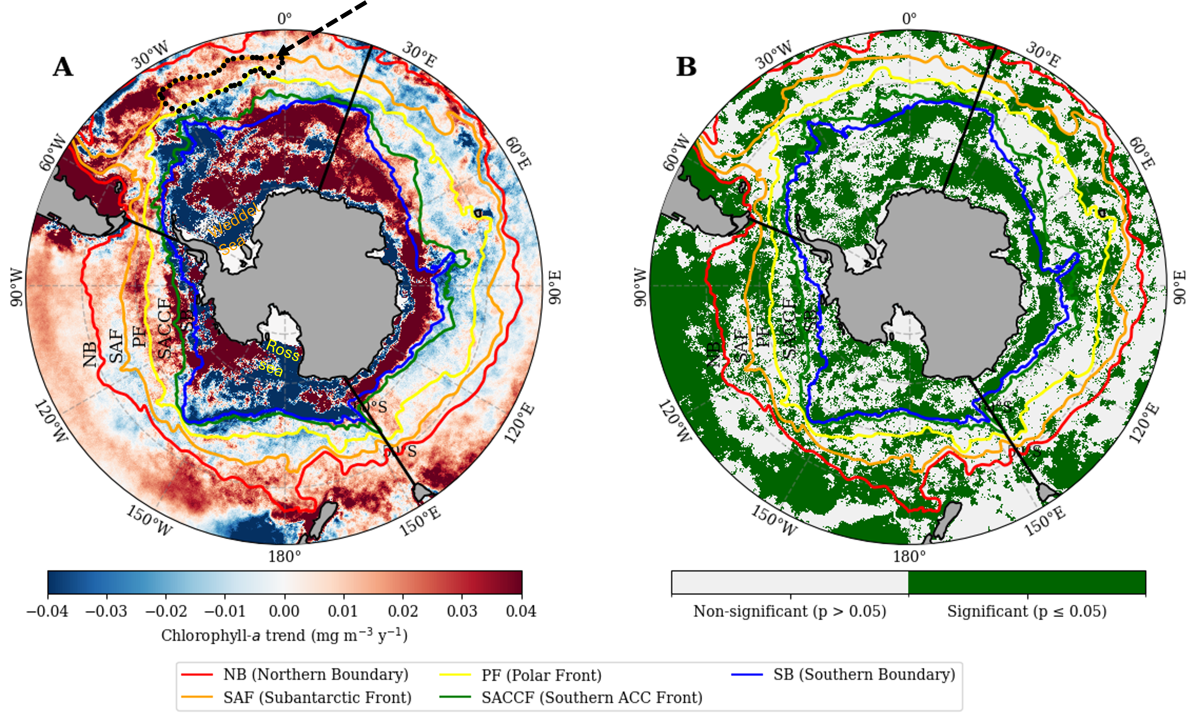
Figure 2.5: Long term trends and their statistical significance for chlorophyll-a concentrations in the Southern Ocean. A) Trends in chlorophyll-a (mg m–3 y–1) derived from the Copernicus Globcolour data (1998–2023). Areas north of the Southern Antarctic Circumpolar Current (ACC) Front with significant positive trends are co-located with other ACC fronts; for instance, along the Subantarctic Front in the Atlantic sector (dotted black line, dashed black arrow). B) Significance map of the trend at the 5% confidence level.
The time series of annual average Chl-a concentrations for the 26 years examined are displayed in Figure 2.6 for the various inter-frontal regions and the entire Southern Ocean. They confirm that during this period the Chl-a concentration generally decreased going northward from the Antarctic continent, reaching minimum values in the SAF–PF region (yellow curve in Figure 2.6A), and then increased again in the NB–SAF region. A remarkable feature in most areas is the observed 5–6-year cycle, which was most pronounced for the SB–AntCoastline and SACCF–SB regions, with relative minima in 1998, 2002, 2008, 2013 and 2018. The latter year is also when the lowest annual Chl-a values were observed over the 26 years for the entire Southern Ocean and most of its sub-regions, while the highest annual values were in 2010 (for instance, 0.51 mg m–3 for the SB–AntCoastline area). Relative minima in Chl-a are observed in various years, such as SAF–PF and PF–SACCF in 2002, NB–SAF and SACCF–SB in 1998, and SB–AntCoastline and the entire Southern Ocean in 2018. The time series for all inter-frontal regions overall follows a remarkably similar pattern, which seems to indicate that large-scale forcings are at play to drive the interannual variability across these regions.
Significant positive trends are shown for the 40°S–NB (p = 0.004), NB–SAF (p = 0.027) and SAF–PF (p = 0.015) regions (Figure 2.6B–D). The trends are not statistically significant (p > 0.05) for the other regions (Figure 2.6E–G). For the SB–AntCoastline region, however, the non-significant trend is the result of significant positive and negative changes in its eastern and western sectors that cancel each other out. When Figure 2.6G was split into these two sectors (not shown), a statistically significant positive trend was observed in the east and a negative one in the west. The total number of valid Chl-a observations in each inter-frontal region for each of the 26 years examined shows some variability (Figure S2), yet the pattern of this variability did not show any relationship to the variability observed for Chl-a.
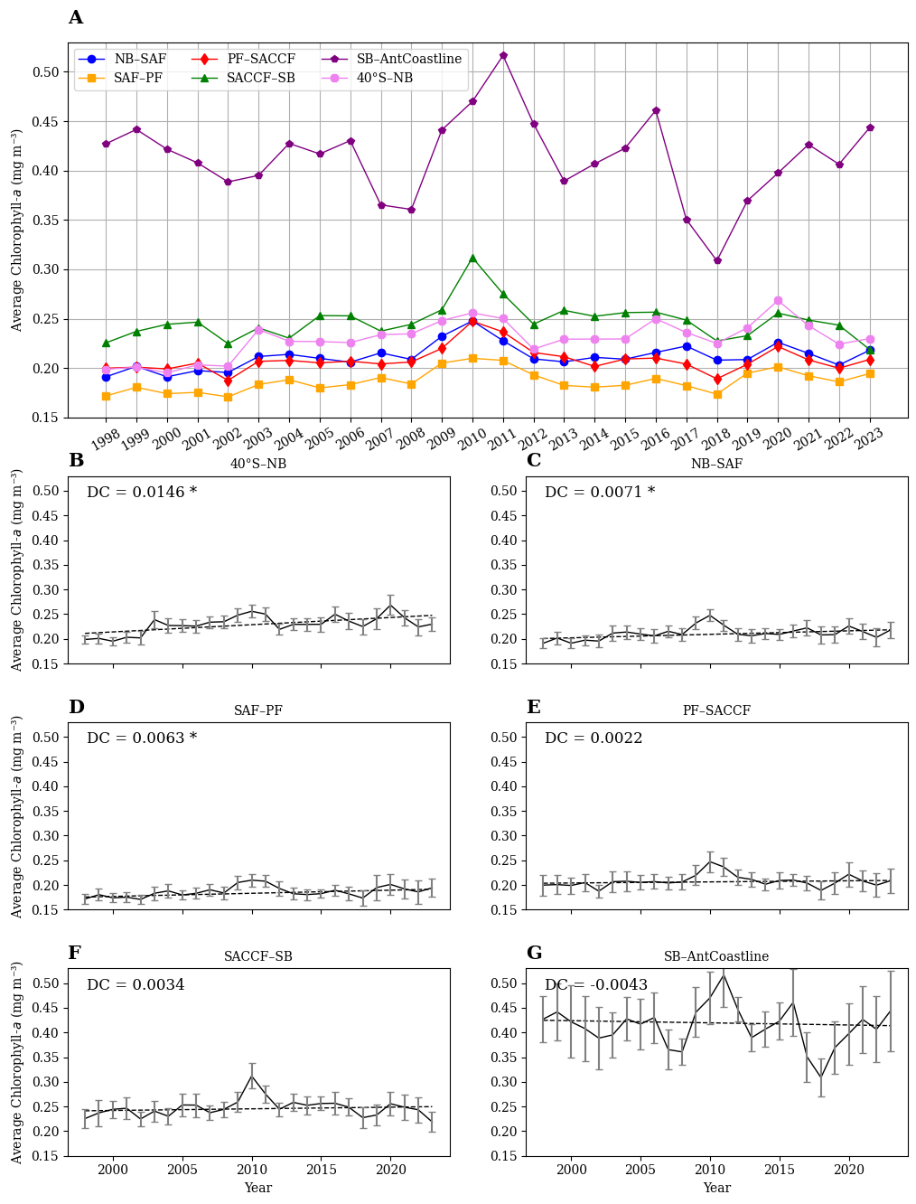
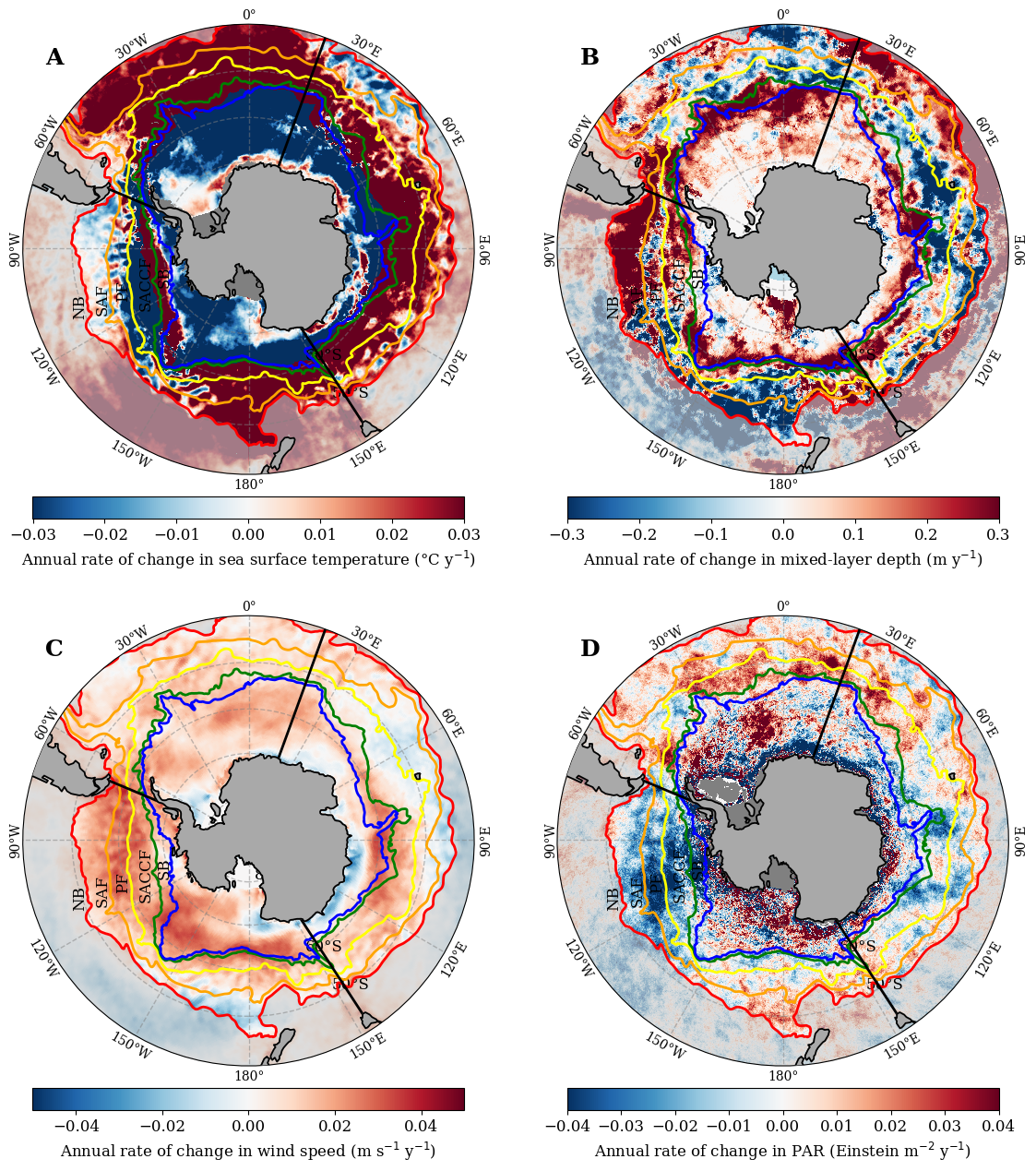
Figure 2.7: Annual rate of change of different physical variables in the Southern Ocean. Annual rate of change over 1998 to 2023 for A) sea surface temperature, B) mixed-layer depth, C) wind speed, and D) photosynthetically available radiation (PAR). The colour-coded contours indicate the mean positions of the fronts (where ACC refers to Antarctic Circumpolar Current). Maps of the statistical significance of these trends are provided in Figure S3.
We performed the same analyses carried out on Chl-a for the four identified potential physical drivers of phytoplankton distributions, SST, MLD, PAR and WS. The temperature trend (Figure 2.7A) shows that the SB–AntCoastline region and the low-latitude regions between 40ºE and 60ºE in the Indian sector and south of Australia were cooling over the 26 years considered here. In contrast, the areas from the PF to the north, especially in the Pacific and Atlantic sectors of the Southern Ocean, were warming. The temperature trend across the Indian sector is patchy. Some of the areas within the SB–AntCoastline that show significant cooling are also where strong positive changes in Chl-a occurred, indicating in these situations a strong inverse relationship between SST and Chl-a.
The MLD trend (Figure 2.7B) represents the rate of change in MLD over the 26-year period. A positive trend(increasing MLD or deepening) is observed in 69% of the Southern Ocean, especially in the region between the SB and Antarctic coastline and in the coastal waters of South Africa along the NB front. On the other hand, a negative trend (i.e., decreasing MLD or shoaling) is observed in the Pacific sector of the Southern Ocean within the region from 40ºS to NB. The MLD also became shallower north of NB in the Pacific and Atlantic sectors during this 26-year period, while Chl-a increased in that area.
The WS (Figure 2.7C) strengthened in the region between the SB and Antarctic coastline, especially in the Pacific sector, and in most parts of the Atlantic sector. Conversely, weaker winds were observed in the Pacific sector within the region of 40ºS to NB and near the western Australian portion of the Indian sector and close to the New Zealand Coast.
Lastly, PAR (Figure 2.7D) shows increases in the region between the Antarctic coastline and the SB region, and mostly in the Atlantic sector of the Southern Ocean. On the other hand, a decreasing pattern appeared in the region close to Tasmania and beyond the NB in the Indian sector.
2.4.3 Concomitant changes of Chl-a and its physical drivers
The physical variables we selected (SST, MLD, PAR and WS) can influence phytoplankton growth either positively or negatively. Accordingly, their intermingled influences can lead to increases or decreases in the satellite-derived chlorophyll concentration. Therefore, we compared the direction of change of Chl-a and of the four physical variables over the 26 years examined, then quantified the degree of correlation of their time series using monthly anomalies, and finally attempted to identify which of the four variables was associated most strongly with the long-term changes of phytoplankton in the Southern Ocean.
2.4.3.1 Directions of change
Results are displayed in Figure 2.8, where trends of the same sign are depicted in green when both Chl-a and the other variable increased and blue when both decreased, and trends of opposite signs are in yellow when Chl-a increased and orange when it decreased. Results are presented here for areas of the Southern Ocean south of the NB; accordingly, lower latitude areas were grey-shaded on the figure.
About 25% of the Southern Ocean showed concomitant Chl-a and SST increases (green in Figure 2.8A) during this 26-year period. In 19% of the ocean, both variables decreased (blue); for instance, from the SB to the Antarctic coastline in the Pacific sector.
For the MLD (Figure 2.8B), the distributions of areas of concomitant and opposite trends with Chl-a often mirrored that for SST. Exceptions include the northern region of NB–SAF within the Pacific sector, where Chl-a and SST exhibited simultaneous increases (green) whereas Chl-a and MLD showed an opposite pattern, with Chl-a increasing and MLD decreasing (yellow). Overall, 37% of the Southern Ocean showed increases in both Chl-a and MLD, and 15% experienced decreases in both. An inverse pattern was observed in 21% of the total area, where Chl-a increased as MLD decreased.
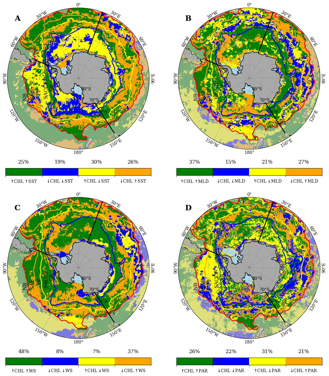
The Chl-a-WS relationship (Figure 2.8C) showed similarities to the one observed for Chl-a and MLD, albeit with some variations. For instance, in the northern part of NB–SAF, Chl-a decreased as WS increased (yellow). Approximately 48% of the Southern Ocean showed simultaneous increases in both Chl-a and WS, while only 8% of the area exhibited decreases in both variables. Additionally, 7% of the area showed an increase in Chl-a with a decrease in WS.
The Chl-a-PAR relationship (Figure 2.8D) indicates that 26% of the areas exhibited parallel increases in both Chl-a and PAR, while 22% showed concurrent decreases. Conversely, 31% of the areas displayed an opposite pattern, where Chl-a increases as PAR decreases, predominantly in the Pacific and Atlantic sectors of the Southern Ocean. The remaining 21% of areas showed decreasing Chl-a alongside increasing PAR.
2.4.3.2 Correlation of the time series of monthly anomalies
We found a strong positive correlation between Chl-a and SST (Figure 2.9A) in the Antarctic coastal region and the region between the NB and SAF. Negative correlations were observed for lower latitudes (below about 45°S), especially in the Atlantic and Indian sectors. On a broader scale, around 60% of the Southern Ocean exhibited a positive correlation between Chl-a and SST.
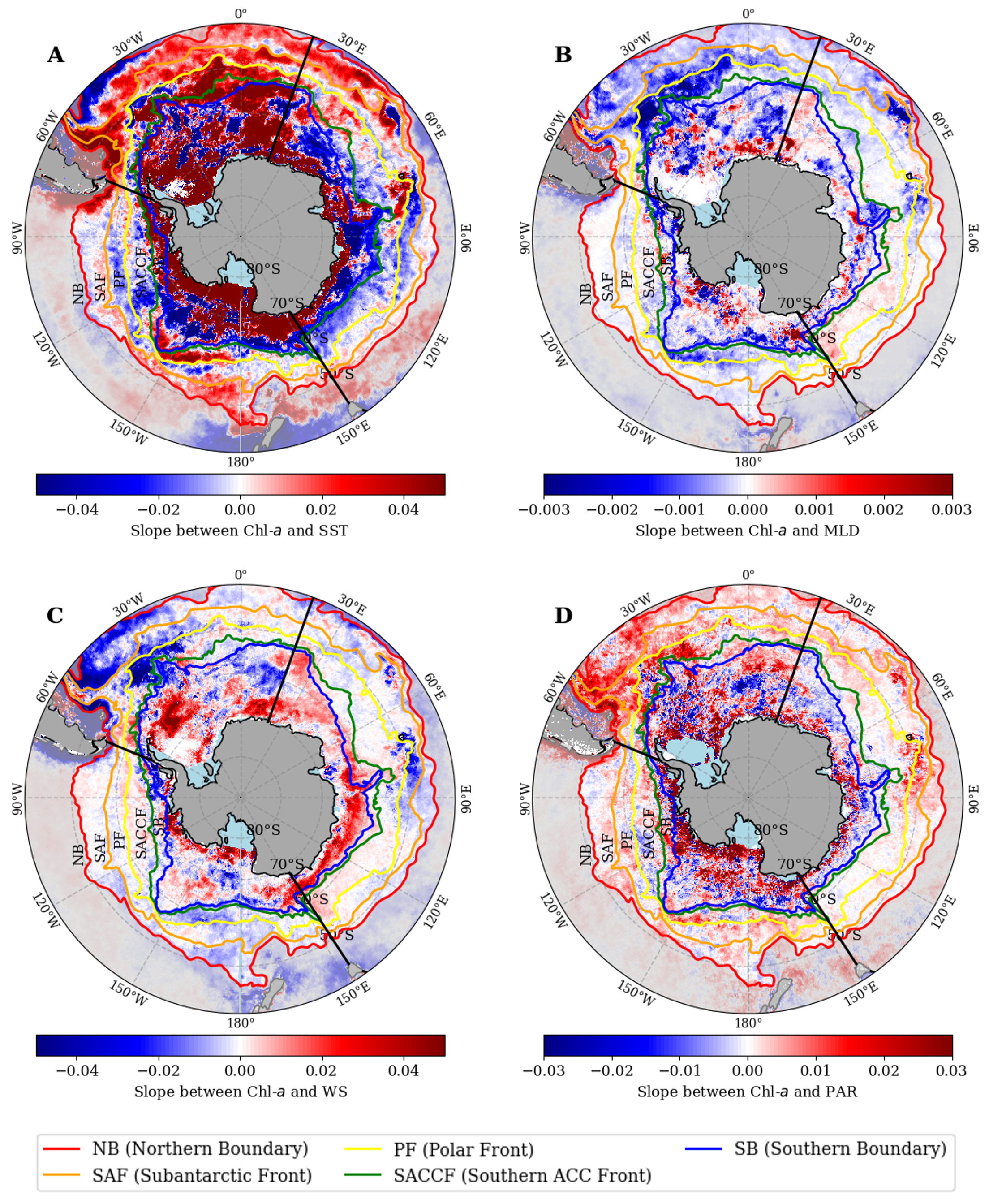
Figure 2.9B demonstrates the relationship between Chl-a and MLD in the Southern Ocean during the 26-year period examined. The correlation was positive within the latitudinal band ranging from approximately 40ºS to 45ºS in the Pacific sector of the Southern Ocean and the Antarctic coastline. However, the Atlantic sector and the African and East Australian coastal regions showed a strong negative relationship. Overall, positive correlations between MLD and Chl-a were seen in about 32% of the Southern Ocean, with negative correlations in 68% of the area.
The relationship between Chl-a and WS in the Southern Ocean during this period was generally weak (Figure 2.9C) in the regions of NB–SAF, SAF–PF and PF–SAF in the Pacific and Indian sectors, except in the coastal region beyond of the NB and SB–AntCoastline region. Roughly half the Southern Ocean showed a positive correlation between Chl-a and WS. Chl-a was linked positively with PAR in two-thirds of the Southern Ocean, except for a slight negative association near the SB along the latitude band of 60°S (Figure 2.9D).
2.4.3.3 Dominant physical driver
To further assess which of the four physical variables had the strongest relationship with Chl-a over the 26-year time series, we normalized the monthly anomalies to their minimum and maximum values. We then calculated the coefficient of determination of their relationships (R2) to understand which variable was most associated with the long-term changes of Chl-a in the Southern Ocean. Results are displayed in Figure 2.10.
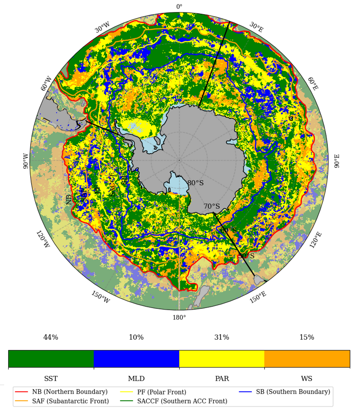
Based on this method, of the four physical drivers considered SST emerged as the dominant factor associated with the changes in Chl-a. SST explained approximately 44% of the Chl-a variance across the Southern Ocean. MLD exhibited the least influence, accounting for only 10% of the variance in Chl-a in the Southern Ocean, as indicated by the low R² value (0.28), especially when compared to other physical variables in the region. The influence of these drivers was observed prominently in the NB–SAF inter-frontal region, as evident in Figure 2.10.
2.4.4 Sensitivity analyses
The comparison between GlobColour and ESA OC-CCI Chl-a data showed that spatial distributions, general seasonal variability, and sector/front differences (Figures 2–4) were largely preserved, although average Chl-a levels were approximately 50% higher in the ESA OC-CCI dataset (Figure S4). Spatial patterns of long-term trends (Figure 2.5) showed little changes, yet trends were higher and statistically significant over a larger proportion of the Southern Ocean when using the ESA OC-CCI data (Figure S5). However, the inter-annual variability obtained from each data set differed, with the ESA-CCI results being less consistent among the various inter-frontal regions and not showing the same 5–6-year cycle as shown in Figure 2.6 using GlobColour. The coefficients of variation of monthly or annual Chl-a values were higher from the ESA-CCI south of the SAF and lower north of it. This pattern seems consistent with the Polymer bio-optical model having been developed using data from low-latitude areas. The comparative directions of change of the Chl-a and physical variables (Figure 2.8) and the results from the linear regression on anomalies (Figures 9–10), however, are remarkably similar, confirming that both Chl-a data sets consistently map areas of long-term Chl-a increase and decrease.
The results from using the seven provinces defined by Ardyna et al. (2017; Figure S6) were very close to the display on Figure 2.6, which confirms that the location and shape of these seven provinces are largely driven by the Southern Ocean fronts. Because these provinces were defined from the phytoplankton phenology (seasonal variations), this result also supports the hypothesis that using inter-frontal regions allows following homogeneous entities over time. When the analysis was repeated using fixed latitude bands of 5 degrees, each starting at 40°S, the results differed significantly (Figure S7). The temporal patterns varied across the various latitudinal bands, in contrast to the consistent patterns observed in Figures 6 and S6.
Finally, regarding sea ice coverage, we estimated the uncertainty introduced by varying ice cover on annual Chl-a values in the SB–AntCoastline region (Figure S8). By recalculating annual means using only ice-free areas, we found that variations ranged between 0.300 mg m–³ and 0.325 mg m–³ (around 10% uncertainty; Figure S8). This result indicates that the changes in annual Chl-a values displayed in Figure 2.6 can be interpreted as reflecting intrinsic interannual variability of Chl-a, and not as artifacts of varying sea ice coverage.
2.5 Discussion
2.5.1 General spatial and temporal variability of phytoplankton in the Southern Ocean
The spatial variability of Southern Ocean phytoplankton that we found for the 26-year period examined (Figures 2–4) largely followed the Southern Ocean fronts and showed significant differences among the Pacific, Indian, and Atlantic sectors, similar to the findings of Ardyna et al. (2017). The same general pattern of Chl-a distribution was documented by Pinkerton et al. (2021), who used 20 years of MODIS data for the Southern Ocean and showed that some regions in the Antarctic coastal zone (Ross Sea, Western Antarctic Peninsula) had high Chl-a values. This pattern was likely explained by polynyas, which are areas of open water surrounded by sea ice that allow phytoplankton to grow (Arrigo et al., 2015). Prend et al. (2022) also found higher Chl-a concentrations around islands or near the Antarctic coastline and in regions outside the NB in the Atlantic and Pacific sectors, particularly between New Zealand and Tasmania where deep water iron fluxes might play a significant role (Boyd et al., 2012; Tagliabue et al., 2014).
Iron availability has been suggested as a driver for the regional variability of Southern Ocean phytoplankton (Boyd et al., 2012; Prend et al., 2022). Our study found the maximum mean Chl-a in the Atlantic sector of Southern Ocean, which was almost twice the value in the Indian and Pacific sectors (Figure 3B). An increased iron availability because of the greater proximity of land might explain this finding (Banse, 1996; Debaar et al., 1995). Studies have shown that the Atlantic sector benefits from natural iron fertilization from continental shelf sources, leading to higher iron concentrations, consequently contributing to the higher phytoplankton biomass (de Jong et al., 2012). In contrast, the Pacific and Indian sectors generally have lower iron availability, which limits primary production (Fourquez et al., 2023; Quéguiner, 2013).
Our study reveals a consistent seasonal pattern in the Chl-a concentrations across the five inter-frontal regions of the Southern Ocean, with peak values observed in summer in the SB–AntCoastline region and relatively steady low values across the ocean in winter. This pattern is in line with the findings of Carranza et al. (2014), who reported elevated satellite Chl-a levels in the Southern Ocean during the summer months due to wind-driven upwelling. In Antarctic coastal waters, the increased sunlight during summer months enhances phytoplankton photosynthesis and growth, leading to higher Chl-a concentrations. This increase in phytoplankton productivity is supported by Deppeler and Davidson (2017), who noted that surface water freshening by ice melt leads to stratification, so that phytoplankton grow in shallow mixed layers with intense light. Further research, however, is needed to fully understand the complex interplay of these physical factors on phytoplankton in different regions of the Southern Ocean.
2.5.2 Long-term changes of phytoplankton and physical variables
The 26-year Chl-a trends revealed significant increases in many parts of the Southern Ocean, with some significant decreases, however, in the Atlantic and Pacific sectors near the Antarctic coast (Figure 2.5A,B). Our findings align with those of Del Castillo et al. (2019), who reported substantial increases in Chl-a concentrations across all regions of the Southern Ocean, with a considerable rise in the area between the northern Pacific and Indian sectors. In these regions, upper-ocean warming and elevated pCO2 levels were predicted to boost the phytoplankton (Boyd, 2019; Steinacher et al., 2010), consistent with the observed increase in Chl-a (Figure 2.5A). The negative trends in the Ross and Weddell seas and along the Antarctic coast in our study echo Pinkerton et al. (2021), while the West Antarctic Peninsula region showed a decreasing pattern in Chl-a, contrasting with the positive trends found by Kim et al. (2018). The observed trends in Chl-a may also be influenced indirectly by other factors, e.g., the larger-scale El Niño Southern Oscillation and the Southern Annular Mode which modulate oceanographic conditions (e.g., MLD, nutrient supply, and light availability) that, in turn, affect phytoplankton dynamics, as well as local-scale factors like glacier melting, sea ice formation, and coastal current patterns (Brown et al., 2019; Kim et al., 2018; Montes-Hugo et al., 2009).
When the entire Southern Ocean is considered, the positive Chl-a trend was not statistically significant, similarly to what was reported by Mishra et al. (2022). In terms of inter-frontal regions, all regions showed a notable increase in Chl-a in the year 2009–2010 and a drop in Chl-a in 2018 (Figure 2.6). Mishra et al. (2022) also found the highest Chl-a concentration in the Southern Ocean in 2010 using satellite data from 2002 to 2015. Globally, the calendar year 2010 was marked by significant deviations (exceeding 40% in many areas) from the long-term average of satellite Chl-a (Blunden et al., 2011). The most notable increase in Chl-a occurred in the Southern Ocean south of 55°S, where phytoplankton bloomed throughout the year.
The cooling trends observed at high latitudes are consistent with the findings of (Auger et al., 2021; Haumann et al., 2020), who reported similar patterns in their studies. The cooling of SST was caused by enhanced upwelling of nutrient-rich deep water which reduced stratification of the water column. Several factors, such as the shift from El Niño to La Niña conditions in the summer and the emergence of a negative Pacific Decadal Oscillation pattern, influenced SST variations in 2010 (Blunden et al., 2011). As shown by Behrenfeld et al. (2006), there is a general inverse relationship between Chl-a and SST, indicating that physical processes play a crucial role in regulating phytoplankton dynamics. This relationship supports the significance of SST as a proxy for light, nutrient availability, and other forcing factors that control global Chl-a concentrations.
The surface cooling (Figure 2.7A) and strong winds (Figure 2.7C) observed between the SB and Antarctic coastline are expected to deepen the MLD (Figure 2.7B), bringing nutrient-rich water to the surface. This process supports phytoplankton growth and significantly increases Chl-a levels in this region (Constable et al., 2014; Deppeler & Davidson, 2017). Over the period of our study, the MLD became shallower north of NB in the Pacific sector, while Chl-a became higher in that area, resulting in opposite trends for MLD and Chl-a (Figure 2.8B). A shallower mixed layer could increase PAR availability for phytoplankton, and higher winds could bring more iron and silicon, which could lead to higher Chl-a levels (Del Castillo et al., 2019). The PAR trend (Figure 2.7D) aligns with the results of Ryan-Keogh et al. (2023) and is attributed to changes in atmospheric cloudiness, as reported by Pinkerton et al. (2021).
2.5.3 Concomitant changes of Chl-a and its physical drivers
We observed predominantly parallel changes (both decreases) in Chl-a and SST in the Pacific sector of the Southern Ocean, specifically within the region from the SB to the Antarctic coast, and opposite changes of Chl-a and SST within the same region in the Atlantic and Indian sectors of this ocean. Beyond the SB, a varied pattern of changes emerged among the other inter-frontal regions of the Southern Ocean (Figure 2.8A). The parallel trends were more common in the Pacific and Atlantic sectors of the Southern Ocean, from the SB to the north, as Carranza and Gille (2015) also found. In addition, Pinkerton et al. (2021) found a strong spatial association between Chl-a and SST for a large region in the Southern Ocean. SST can affect phytoplankton growth directly by changing metabolism (Reay et al., 2001), yet the same association were also related to frontal features, suggesting that ocean circulation and stratification may be the main factors behind these trends. As explained by O’Malley et al. (2010), these concomitant changes show the close link between phytoplankton and their physical surroundings. As for some areas in our study, Behrenfeld et al. (2006) also observed opposite trends between Chl-a and SST in their global ocean analysis. Areas where Chl-a and SST have opposite trends are likely to have upwelling, such as near the Antarctic coast in the Atlantic and Pacific sectors and near the NB in the Indian and Atlantic sectors. As these opposite trends in our study corresponded with higher Chl-a levels, they were likely caused by the upwelling of nutrient-rich, cold waters from below the euphotic zone, due to surface cooling and enhanced wind-mixing (Figure 2.6A), as suggested by Carranza and Gille (2015). In the northern part of NB–SAF, where Chl-a decreased with increasing WS (yellow in Figure 2.8B,C), strong winds would have caused deep mixing, limiting light availability for phytoplankton near the Antarctic coast (Lovenduski & Gruber, 2005). An opposite Chl-a-PAR pattern (yellow in Figure 2.8D), where Chl-a increased despite declining light availability, was evident across a considerable portion of the Pacific and Atlantic sectors. Photoadaptation to low-light conditions may contribute to this opposite pattern (Ryan-Keogh et al., 2023).
2.5.4 Dominant physical drivers
The positive correlation between Chl-a and SST in the SB–AntCoastline region suggests that a shallow, warm mixed layer enhanced the Chl-a levels. Such enhancement is due to the effects of mesoscale eddies and fronts, which can change upper ocean stratification and SST, rather than to decreased wind mixing or surface warming (Fox-Kemper et al., 2008). These dynamics, coupled with turbulent mixing driven by winds and buoyancy forcing, influence the stratification of the surface mixed layer and boost phytoplankton levels (Llido et al., 2005). Pollard et al. (2002) have suggested that stratification and Ekman advection generated by frontal dynamics can lead to an inverse relation between Chl-a and SST, which appears to be consistent with what we observed here between the SAF and PF.
Large areas of the Southern Ocean in the Antarctic coastline region showed significant relationships between Chl-a and WS (Figure 2.9C), indicating that strong winds can impact phytoplankton blooms noticeably (Kahru et al., 2010). Our findings that strong winds led to increased Chl-a in the summer suggest that wind-driven upwelling helps to prolong spring phytoplankton blooms.
Regarding environmental drivers of changes in Chl-a based on the variance explained by the individual variables considered, our analysis found that SST accounted for approximately 44% of the observed variance across the area, making it the primary contributor to Chl-a variability. MLD had the least influence on Chl-a levels. These findings are consistent with Pinkerton et al. (2021), who highlighted the importance of SST in explaining major variations in Chl-a and identified MLD as having minimal impact. Additionally, Krumhardt et al. (2022) found that SST plays a significant role in the ACC region, while PAR influences Chl-a in the sea ice zone in the Southern Ocean. They suggested that changes in Chl-a within the ACC, which is experiencing warming, are influenced by increased iron input and other physical drivers such as temperature and light availability.
2.6 Conclusion
In conclusion, this study has revealed significant spatial and temporal variability in Chl-a concentrations across the Southern Ocean from 1998 to 2023, as observed through Copernicus-Globcolour satellite data. The highest concentrations were found between the SB and the Antarctic coastline, particularly in the Western Antarctic Peninsula and Ross Sea regions, while reduced levels were observed between the PF and SAF and north of the NB. Seasonally, the highest Chl-a levels were recorded during spring for all regions, except for the SB–AntCoastline region where the peak occurred in summer and the lowest across all regions during winter. During this 26-year period, there has been a substantial increase in Chl-a across many parts of the Southern Ocean, with the highest annual average observed in 2010 in the SB–AntCoastline region and a trend cycle of 5–6 years, suggestive of large-scale forcings at play.
Furthermore, the study identified significant environmental influences on Chl-a concentrations. Areas of the Southern Ocean are experiencing temperature changes, with cooling observed in the Antarctic coastal region and warming in areas north of the PF, especially in the Pacific and Atlantic sectors. MLD is deepening and WS is strengthening in most parts of the Southern Ocean, changes that appear to be closely associated with patterns in Chl-a concentration within these regions. Overall, however, SST accounted for approximately 44% of the variance in Chl-a across the Southern Ocean, making it the primary driver, while MLD had the least influence. In our future research, we will explore the relationships between observed annual Chl-a trends and sea ice coverage, as well as larger-scale climate variables like El Niño Southern Oscillation and the Southern Annular Mode.