1 General introduction and literature review
1.1 Scientific Background and Rationale
The Southern Ocean is a critical component of the Earth system because of its disproportionate role in global heat uptake, carbon sequestration, and ocean circulation. Understanding how this region responds to ongoing climate change is therefore of global importance. Central to this response are phytoplankton, microscopic marine organisms that underpin Southern Ocean food webs and drive biological carbon export. The distribution and productivity of phytoplankton are strongly regulated by physical processes, including ocean fronts, temperature, mixed-layer dynamics, circulation, and sea ice. Because many of these physical controls are undergoing rapid change, there is growing concern about how Southern Ocean phytoplankton ecosystems will respond in coming decades. Despite substantial progress, significant uncertainties remain regarding the long-term variability of phytoplankton, the relative importance of different drivers, and their future trajectories under climate change. This chapter reviews the current state of knowledge and identifies the scientific gaps addressed by this thesis.
1.1.1 The Southern Ocean
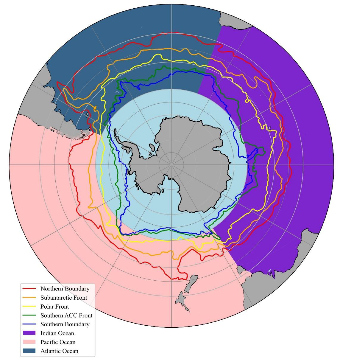
The Southern Ocean (SO) is a broad ocean region encircling Antarctica (Talley, 2013). It is defined as waters south of the Subtropical Front and covers 10-15% of the global ocean (Turner et al., 2009). Its Indian (~30°E-150°E), Pacific (150°E-60°W) and Atlantic (60°W-30°E) sectors are sometimes considered as having specific oceanographic properties (Figure 1.1). For example, the Atlantic sector generally exhibits higher phytoplankton biomass and productivity owing to enhanced natural iron inputs from continental margins and island systems, whereas the Pacific sector is characterised by more extensive iron limitation and lower average productivity. The Indian sector displays strong interactions between the Antarctic Circumpolar Current, mesoscale circulation, and topographic features, producing substantial regional variability. These sectoral differences influence ocean circulation, nutrient availability, sea-ice dynamics, and biological productivity, contributing to the marked spatial heterogeneity observed across the Southern Ocean. The SO is a unique oceanographic environment due to the lack of continental barriers blocking its flow and the strong winds blowing across the surface (Rintoul & Garabato, 2013). It is considered instrumental in the functioning of the global ocean and responsible for over a third of the global uptake of CO2 across the surface, playing a key role in driving global biogeochemistry (Ferreira et al., 2020; Gruber et al., 2009). Since the last century, it has experienced rapid climate change, which has led to significant alterations in this marine ecosystem (Constable et al., 2014; Turner et al., 2009).
The SO plays a critical role in mediating global climate and the carbon cycle, accounting for almost 40% of the anthropogenic carbon uptake in the ocean (Del Castillo et al., 2019; Frolicher et al., 2015; Takahashi et al., 2009). Observations over past decades indicate that this ocean is undergoing increasingly rapid changes in atmospheric and ocean circulation, temperature, sea ice cover, and stratification (Joy-Warren, 2022; Turner et al., 2014). These changes alter the duration and magnitude of primary production (production of organic matter by phytoplankton), as well as the phenology of the phytoplankton community composition of phytoplankton assemblages (Alexander Hayward et al., 2025; Joy-Warren, 2022). Climate change is altering multiple components of the Southern Ocean system. Observations indicate regional warming of surface waters across large parts of the Southern Ocean, while several Antarctic Circumpolar Current fronts have shown evidence of southward displacement in some sectors (Constable et al., 2014; Kim & Orsi, 2014; Sallée et al., 2008). Climate projections suggest further changes in temperature, salinity, mixed layer depth, wind strength, sea ice thickness, upwelling and nutrient replenishment, and glacial ice melt in the SO will continue (Bracegirdle et al., 2013; Meijers et al., 2012; Russell et al., 2006; Sen Gupta & McNeil, 2012). These physical and chemical changes largely control the plankton habitats of the Southern Ocean by modifying the availability of light and nutrients (Johnson et al., 2013). Increased stratification, triggered by surface warming and freshening, will lower phytoplankton access to the nutrients below the mixed layer and increase the mean mixed layer irradiance. The impacts of increased stratification are expected to vary spatially across the Southern Ocean. In regions where phytoplankton growth is primarily limited by light availability, particularly at high latitudes, shallower mixed layers may enhance productivity by increasing the mean light exposure experienced by phytoplankton. In contrast, in regions where nutrients become limiting, stronger stratification can reduce vertical nutrient resupply from deeper waters and constrain phytoplankton growth. Consequently, many model projections suggest declining net primary production across large areas of the Southern Ocean, while some regions, including parts of the Subantarctic Zone and Antarctic Circumpolar Current system, may experience stable or enhanced productivity due to improved light conditions and regional differences in nutrient availability(Arrigo et al., 2008; Boyd et al., 2008). Such rapid changes to the fundamental components of the Southern Ocean will have consequences for all levels of the polar ecosystem.
Shifts in primary production will significantly alter regional and global nutrient cycling, organic carbon and biogenic silica export (Assmy et al., 2013), carbon drawdown (Moreau et al., 2012), grazing communities and higher trophic levels (Saba et al., 2014), and benthic-pelagic coupling (energy and nutrient transfer from the pelagic to the benthos) (Assmy et al., 2009). Marine mammals and birds are expected to have significant changes to the energy they need to spend to get to food and more prolonged or complex foraging trips for those bound to breed large scales (Constable et al., 2014). If the ecosystem cannot adapt rapidly enough, there will be a decline in abundance and loss of biodiversity and ecosystem functions in the future.
1.1.2 The Southern Ocean phytoplankton
1.1.2.1 Marine phytoplankton and primary productivity
Phytoplankton are crucial for Antarctic food webs dynamics and regulating global climate through ocean biogeochemical cycles (Deppeler & Davidson, 2017). These microalgae occupy the sunlit surface layer of the ocean. They fuel the oceanic food web and regulate oceanic and atmospheric carbon dioxide levels through the photosynthetic carbon fixation process (Martinez, Brini, et al., 2020). Globally, more than 100 million tonnes (40–50%) of inorganic carbon are fixed by phytoplankton per day (Behrenfeld et al., 2006; Field et al., 1998), although the phytoplankton biomass equates to less than 1% of the total photoautotrophic biomass estimated on the planet (Bryant, 2003). This organic carbon is transferred through the food web, exported to the deep ocean through what is called the biological pump (Basu & Mackey, 2018), and ultimately a tiny fraction is buried into sediments. The efficacy of the biological pump is a function of phytoplankton physiology and community structure, which are governed by the ocean's physical and chemical conditions (Petrou et al., 2016). Phytoplankton encompass a wide range of organisms highly diverse in size and shape. About 350 phytoplankton species (e.g., diatoms, dinoflagellates, green algae, coccolithophores, cyanobacteria, etc.) are found in Antarctic waters among the 500 identified protists (Harris, 2006). These microscopic plants of the upper ocean are vital to the health and productivity of the marine ecosystem (Buesseler, 1998; Garibotti et al., 2003; Petrou et al., 2016).
1.1.2.2 Phytoplankton functional groups and community composition
Phytoplankton Functional Types (PFT) are conceptual groupings of phytoplankton species which have an ecological functionality in common either in terms of the food web or of their biogeochemical role (IOCCG, 2014). Phytoplankton are often grouped according to their cell size: pico- (0.2-2.0 μm), nano- (2.0-20 μm) and micro-phytoplankton (20-200 μm) (Knox, 2007). In the SO, picoplankton and nanoplankton make up 10-20% and 25-75% of the entire plankton communities (Hewes, 2009). Large-scale spring blooms are dominated by microplankton, including many diatoms, dinoflagellates, silicoflagellates, and Phaeocystis antarctica (a haptophyte) (Alvain et al., 2005; Alvain et al., 2008; Knox, 2007). Dominant species include the diatoms Nitzschia cylindricus and N. pseudonana, although >100 species of diatoms and >60 species of dinoflagellates and silicoflagellates have been recorded from the SO (Knox, 2007; Stonehouse, 2002).
1.1.3 Physical drivers of the Southern Ocean environment
Phytoplankton concentration in the SO is affected by light, temperature, nutrient variability, and the presence of light. In addition, large-scale climatic variables, such as the Southern Annular Mode (SAM) and El Niño events, influence the distribution and concentration of phytoplankton in the SO (Alvain et al., 2008; Arrigo et al., 2008; Behrenfeld et al., 2006; Deppeler & Davidson, 2017; Petrou et al., 2016). Furthermore, oceanographic variables, such as, polar fronts and currents (Arrigo et al., 2008; Knox, 2007; Mann & Lazier, 2013), seawater circulation (Deppeler & Davidson, 2017; Morley et al., 2020), mesoscale eddies and gyres (Deppeler & Davidson, 2017; Knox, 2007; Mann & Lazier, 2013), and upwelling (Mann & Lazier, 2013) all affect the phytoplankton concentration in the SO.
1.1.3.1 The Southern Ocean fronts
Ocean fronts are sharp boundaries between distinct water masses characterised by strong horizontal gradients in temperature, salinity, and density, which are frequently detectable through changes in sea surface temperature (SST) or surface height (SSH) (Chapman et al., 2020). Fronts play a vital role in the distribution of globally essential nutrients (i.e., nitrates) (Palter et al., 2013). Enhanced vertical exchange between the deep and surface ocean occurs in the frontal region, which increases the nutrient concentration of surface waters and influences the phytoplankton community and primary productivity (Mishra et al., 2020). Frontal waters have higher primary production rates than those found in surrounding waters. More precisely, phytoplankton blooms occur where fronts interact with topography and when the divergence of currents brings nutrient-rich water to the surface (Arrigo et al., 2008). For instance, the Polar Front affects the ecological boundaries of phytoplankton communities and prevents poleward introductions (Boyd, 2019; Knox, 2007).
The position of Antarctic Circumpolar Current (ACC) fronts is sensitive to changes in atmospheric forcing due to large-scale climate modes such as El Niño/La Niña (Kim & Orsi, 2014; Sallée et al., 2008). Evidence from climate change shows strong westerly winds are intensifying, and ACC fronts are migrating to the south (Fyfe & Saenko, 2006). Based on about 15 years of satellite altimetry observations (from 1993 onwards), several studies reported that the main fronts of the Southern Ocean had generally shifted south by about 0.5–1.5° (60 km on average) (Kim & Orsi, 2014; Sallée et al., 2008; Sokolov & Rintoul, 2009). This southward migration of ACC fronts may change the structure and environmental conditions of the Southern Ocean’s bioregions and the distribution of nutrients and phytoplankton that form the base of the trophic web (Constable et al., 2014; Deppeler & Davidson, 2017).
As fronts are of fundamental importance to the climate system, scientists are trying to define them in various ways. Still, there is a debate on how many fronts are in the SO. From the ‘traditional view’ of SO, three fronts (subantarctic, polar and southern ACC fronts) are determined by the researchers from research cruises over many decades. This three-front view is supplemented by adding Subtropical front (STF) to the north and Southern Boundary (SB) front close to Antarctica. However, SB and STF are not often regarded as part of ACC fronts due to their distinct dynamics from the ACC fronts(Sokolov & Rintoul, 2007). In the beginning, Orsi et al. (1995) identified five circumpolar fronts, i.e., the southern boundary front, the southern ACC front, the polar front, the sub-antarctic front and the sub-tropical fronts, in the SO using historical hygrographic data and applying water mass criteria (Figure 1.2:B). Later, Park and Durand (2019)discovered that altimetry-derived ACC fronts, which are more realistic of current frontal locations, exist in SO (Figure 1.1). Furthermore, Sallée et al. (2008)also brought up the fact of dynamic ACC fronts, which is also altimetry-derived and are thought to be very useful for checking the long-term variability of phytoplankton between the frontal zones in the SO (Figure 1.2:A).
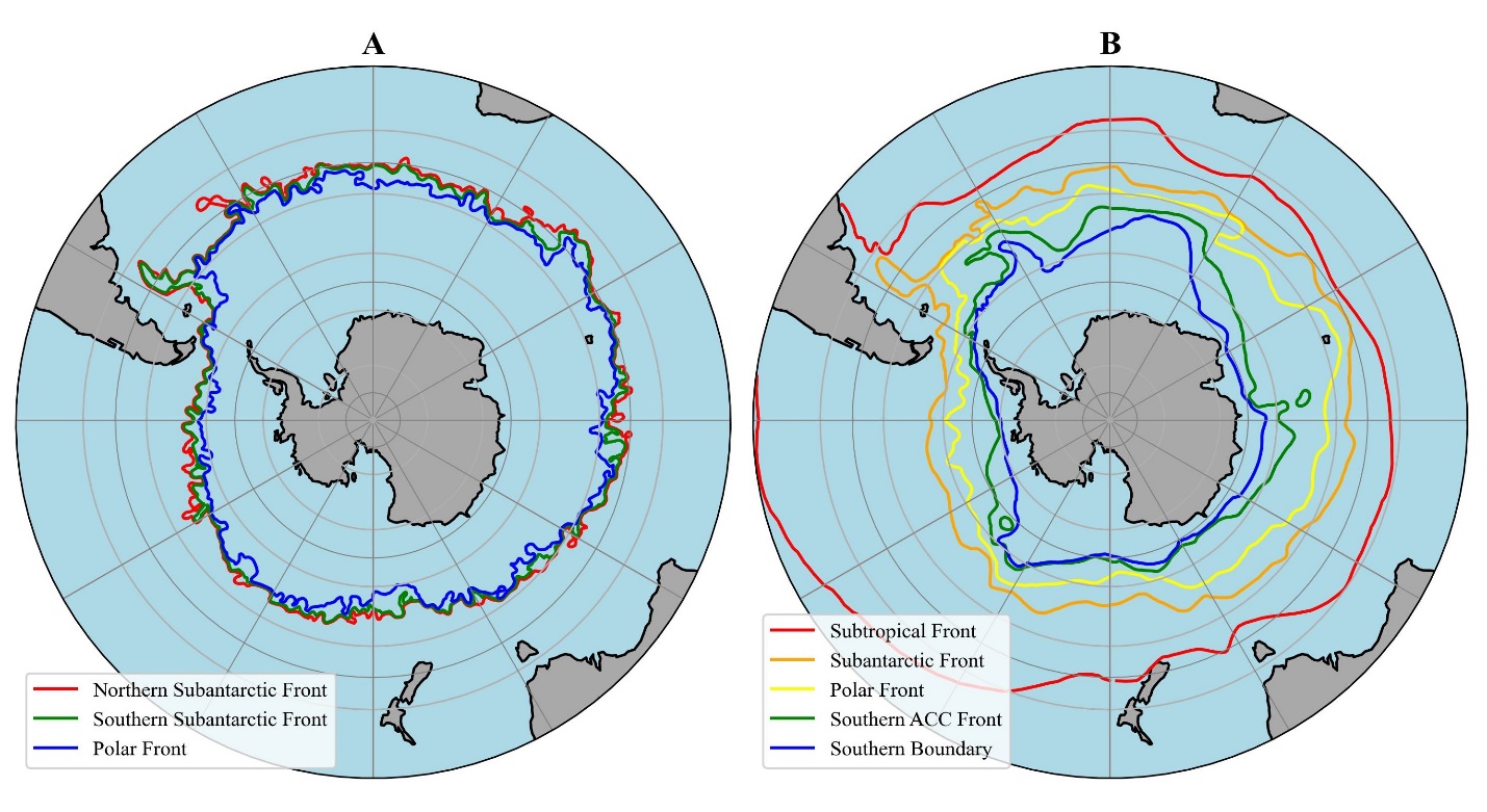
Figure 1.2: The Antarctic Circumpolar Current (ACC) and it’s fronts. A, Weekly snapshot (23 July 2018) of the fronts determined by (Sallée et al., 2008). B, Continuous, smooth and circumpolar fronts determined by (Orsi et al., 1995).
Southern Ocean fronts have significant implications for the physical oceanography of this region and the entire climate system. For example, enhanced density gradients near the fronts support strong oceanic jets via thermal wind (Chapman et al., 2020). Frontal jets are responsible for most of the ACC transport and act as barriers to horizontal mixing (Garabato et al., 2011). Frontal regions are also associated with the exchange between the deep and surface ocean through the upwelling (rising) of deeper waters and downwelling (descending) of surface waters (Morrison et al., 2015). In addition, fronts help to catalyse the generation of mesoscale ‘eddies’(Williams et al., 2007) and sub mesoscale ‘filaments’, which can bring nutrients from the deep ocean to the surface water where they can be consumed by biological components of the system (Levy et al., 2018).
1.1.3.2 Large scale climate drivers: ENSO/SAM
The Southern Annular Mode (SAM), also referred to as the Antarctic Oscillation, is the dominant climate mode of atmospheric circulation in the southern hemisphere (Kidson, 1999; Thompson & Solomon, 2002).
It is defined as the alternating pattern of strengthening and weakening westerly winds in conjunction with high- to low-pressure bands between the mid to high latitudes (Ho et al., 2012). The 'positive' phase of SAM is when pressures are low over Antarctica and high over Australia and New Zealand. SO has seen an increase in the positive phase of SAM during the last 60 years, strongly related to the depletion of the ozone layer over Antarctica and increased concentrations of greenhouse gases (Polvani et al., 2011; Solomon et al., 2005).
On the one hand, it has been predicted that the positive phase of SAM will continue to deepen the summer mixed layer and increase cloud cover, which may result in decreasing phytoplankton biomass and productivity in the permanently open ocean zone (Leung et al., 2015). On the other hand, the intensified jet and its southward shift enhance the Ekman transport equatorward. The sea surface temperature (SST) decreases with more robust Ekman pumping, which may increase phytoplankton biomass in the subantarctic region (Lovenduski & Gruber, 2005; Thompson et al., 2011).
The El Niño–Southern Oscillation (ENSO) is another leading driver of climate variability within the Pacific sector of the SO, involving warm (El Niño) and cold (La Niña) episodes with a typical periodicity of 2–5 years (Clarke, 2008). The ENSO has both positive and negative impact on phytoplankton, primary production, and timings of initiation, peak, termination and duration of the growing period (Racault et al., 2017). Phytoplankton growth in the SO is closely related to long periods of above-average temperatures, conditions typical of El Niño events. On the one side, El Niño transitions (during 1997–1999) are associated with monthly Chl-a anomalies, causing a 10 % increase in phytoplankton biomass globally (Behrenfeld et al., 2001) due to the upwelling of nutrient-rich waters (Behrenfeld et al., 2006). On the other side, Clarke (2008) reported weaker upwelling on the Peru coast because of a deeper thermocline in the region, resulting in decreased phytoplankton biomass, during the strongest El Niño observed in 1982. Scientific studies have yet to fully explore the influence of the ENSO on the SO phytoplankton, which is one of the motivations to work in this region. Therefore, the impact of ENSO in the SO is currently lacking and requires further investigation.
1.1.3.3 Temperature
Temperature is one of the strongest drivers that affects phytoplankton and primary productivity in the ocean by regulating the distribution and abundance of phytoplankton in both spatially and temporally (Petrou et al., 2016). It influences cellular processes, such as cell size, growth, carbon and chlorophyll content with other nutritional requirement in phytoplankton (Boyd, 2019).
In the SO, climate change, e.g., ocean warming, affects the phytoplankton community significantly (Takao et al., 2020). The temperature rise promotes phytoplankton growth and may accelerate sea ice retreat, changing the timing and magnitude of bloom onset in this highly productive region (Deppeler & Davidson, 2017). Such changes result in a temporal mismatch of phytoplankton and higher trophic levels, carbon uptake and ecosystem productivity. Literature review indicates that rising temperatures cause increased grazing rates more rapidly than phytoplankton growth rates in the Sub Antarctic Zone (SAZ) of SO (Behrenfeld, 2014; Evans et al., 2011; Sarmento et al., 2010). In this region, phytoplankton may be low at higher temperatures due to rapid consuming of phytoplankton by the grazers. In addition, Boyd et al., (2013) mentioned that polar diatom shows a 25% increase in growth with the temperature rise by 3◦C.
In Antarctica, Deppeler and Davidson (2017) reported strong variation in temperature patterns between East and West Antarctica, with significant warming in West Antarctica and a slight cooling trend over East Antarctica. Over the last 50 years, greater dominance of cryptophytes over diatoms has occurred in the coastal waters along the west Antarctic Peninsula (WAP), which is among the most rapidly warming regions on Earth (Turner et al., 2005), and this is assumed to be a response to regional warming (Moline et al., 2004).. Montes-Hugo et al. (2009) reported a significant change in Chl-a concentrations from 1978 to 2006 along the WAP using satellite and in-situ data, followed by changes in the dominant phytoplankton community associated with rapid regional climate change along the WAP. In recent times, Brown et al. (2019) found an almost five-time increase in summer oceanic CO2 uptake from 1993 to 2017 along the WAP with changes in phytoplankton dynamics (i.e., biomass and community composition). It is predicted that future increases in sea surface temperature will likely accelerate the melting of ice shelves, increasing the input of fresh, stratified, iron-rich water to polynyas and increasing productivity (Deppeler & Davidson, 2017).
1.1.3.4 Mixed layer depth
The mixed layer depth (MLD) is one of the most important physical controls on Southern Ocean phytoplankton. Mixed layers regulate the balance between light availability and nutrient supply. Deep mixed layers entrain nutrient-rich waters into the upper ocean but expose phytoplankton to reduced average light conditions. In contrast, shallow mixed layers increase light availability but can restrict nutrient replenishment from deeper waters. Consequently, phytoplankton growth in the Southern Ocean is often influenced by the interaction between stratification, light limitation, and nutrient availability. Climate-driven changes in MLD are therefore expected to play a major role in shaping future phytoplankton productivity and community composition.
1.1.3.5 Sea Ice
Sea ice is a defining feature of the Southern Ocean and exerts strong control on phytoplankton productivity through its influence on light availability, stratification, and nutrient cycling. Seasonal sea-ice advance limits light penetration and suppresses phytoplankton growth, whereas sea-ice retreat promotes bloom development by increasing light exposure and introducing freshwater that stabilises the upper ocean. Sea ice can also influence iron supply through meltwater processes and interactions with coastal ecosystems. Recent observations suggest substantial changes in Antarctic sea-ice extent and seasonality, raising concerns about their consequences for Southern Ocean productivity, ecosystem structure, and carbon sequestration.
1.1.3.6 Sea-water circulations and exchange
The SO contains two essential circulation features- the Antarctic Circumpolar Current (ACC) and part of Meridional Overturning Circulation (MOC) (Cunningham, 2005). These two features are responsible for storing and transporting heat, salt, CO2, nutrients and other substances around the globe. The ACC drives the zonal circulation of the SO, flows eastward and connects the southern part of the Atlantic, Indian and Pacific oceans (Rintoul & Garabato, 2013). The MOC connects all ocean basins through a large-scale system of surface and deep currents (Schmittner et al., 2013).
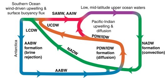
In a simplified zonally-averaged framework (Figure 1.3) described by Rintoul and Garabato (2013); Talley (2013), the three northern currents, i.e., North Atlantic Deep Water (NADW), Indian Deep Water (IDW) and Pacific Deep Water (PDW), rise into the mixed layer in the SO to form the Circumpolar Deep Waters (CDW). Due to the low density compared to NADW, IDW and PDW upwell above and north of the NADW and transform into the upper CDW (UCDW). Part of the UCDW then flows northward by Ekman transport across the ACC and forms the Subantarctic Mode Water (SAMW), an essential source of nutrients for the global oceans. The densest portion of the SAMW further transforms into the Antarctic Intermediate Waters (AAIW). Another part of the poleward-flowing NADW is transformed into lower circumpolar deep water (LCDW) that, denser than UCDW, upwells further south near the Antarctic coast. Here, cooling from air-sea fluxes and salinification from brine rejection transforms LCDW into AABW, particularly in the Weddell and Ross Seas polynyas. The AABW flows northwards until it rises into IDW, PDW and NADW in the subtropics (Talley, 2013).
1.1.3.7 Mesoscale eddies and gyre
An eddy is formed when water currents adopt a circular or swirling motion. This ocean flow pattern at the mesoscale can be hundreds to thousands of kilometres wide, with a surface velocity of greater than 30 cm per second (Knox, 2007; Williams & Follows, 2011). For example, 'turbulent rings', formed by the western boundary currents in the SO, can stimulate phytoplankton bloom formation because the turbulence counteracts the tendency for their dense silica cell wall to sink out of the photic zone (Mann & Lazier, 2013). Mesoscale eddies significantly affect phytoplankton dynamics in the SO. In the Southern Hemisphere, anticyclonic eddies cause upwelling of nutrient-rich waters, enhance stratification, and create ideal conditions for phytoplankton blooms. Alternatively, cyclonic eddies result in downwelling in their core and transport cool, low-salinity water across the Polar Front and the Sub-Antarctic Front (Deppeler & Davidson, 2017; I. Frenger et al., 2018). These processes strongly affect the local growth rate and loss of phytoplankton biomass.
Similarly, gyres are a larger system of circulating currents around the periphery of the ocean basins. Gyres are formed by wind patterns, Coriolis Effect, planetary velocity, and vertical and horizontal friction (Knox, 2007). Gyres circulate water around the entire planet and regulate SST and nutrient concentrations. More specifically, two gyres (Weddell Sea and Ross Sea gyres) circulate above the continental shelf in the SO; (Townsend, 2012; Williams & Follows, 2011). Although the ACC is a closed circuit, it joins the southernmost extent of the major oceanic gyres of the South Atlantic, South Indian and South Pacific (Garrison et al., 2022).
1.1.3.8 Upwelling and nutrient supply
Upwelling, a type of vertical current characterised by high nutrient concentrations, can facilitate high phytoplankton production (Boyce et al., 2010). Upwelling zones are a source of nutrient-rich, cooler, deep water that enters the epipelagic photic zone and is, therefore, sometimes referred to as "the heart of the productivity of the oceans" (Townsend, 2012). Upwelling provides ideal growth conditions when followed by calm high-light periods. During the calm period, stratification in the water column develops due to the warming of the surface waters and reduced salinity if sea ice is melting. This process facilitates phytoplankton on growth and biomass accumulation within the shallow stratified upper layer (Sokolov, 2008).
Wind-driven coastal upwelling occurs when strong winds generate waves, and the water is dragged along the surface as a current. During Ekman transport, momentum is transferred between layers of moving water, and Coriolis force deflects each successively deeper layer farther to the left (in the Southern Hemisphere), creating an Ekman spiral (Mann & Lazier, 2013; Townsend, 2012). When this process occurs away from a coast, surface waters move off-shore and are replaced by nutrient-rich, cooler, deeper water (Knox, 2007; Mann & Lazier, 2013). Thus, upwelling affects the phytoplankton concentration in the SO.
Before examining patterns of phytoplankton variability in the Southern Ocean, it is important to understand how these organisms are observed at basin scales. Because direct observations remain spatially and temporally limited across much of the Southern Ocean, satellite ocean-colour remote sensing has become the primary tool for monitoring phytoplankton biomass and productivity. The following section briefly introduces the principles of ocean-colour radiometry and its application to phytoplankton observations.
1.1.4 Observing Phytoplankton from Space
1.1.4.1 Ocean Colour Radiometry (OCR)
Satellite “Ocean colour radiometry” (OCR) refers to measurements of radiometric quantities at the top of the atmosphere (TOA), typically measurement of the total radiance exiting the ocean+atmosphere system (\(L_{T}\), W m-2 sr-1). From these measurements, one can derive the water leaving radiance (Lw), which can be converted into the remote sensing reflectance (Rrs). This is passive remote sensing, where the sunlight backscattered by the ocean and atmosphere is recorded in a number of spectral bands. The measured signal includes the footprint of absorption and scattering that occurred through the atmosphere and ocean. As for the atmosphere, the processes are scattering by air molecules and aerosols and absorption by atmospheric gases. In the oceans, the processes are scattering by water molecules and particles of biogenic (phytoplankton) or mineral (sediments) origins, and absorption by water molecules, phytoplankton, and Coloured Dissolved Organic Matter (CDOM).
The changes in ocean colour related to these processes were initially described by (Morel & Prieur, 1977). The proportion of the incoming light that is eventually backscattered out of the ocean and is finally measured by the satellite is small and represents less than 10% of the total signal measured at TOA (and often less than 5%). It is therefore necessary to subtract the effects of the atmosphere to get to the water leaving radiance from the signal received by the satellite sensor.
The water leaving radiance (\(L_{w}\)) therefore contains the information about the concentration and optical properties of phytoplankton, suspended particles, and coloured dissolved organic matter (CDOM or gelbstoff) within the upper ocean (Figure 1.4). Differences in how these constituents absorb and scatter light alter the spectral signature measured by satellite sensors, allowing the retrieval of variables such as Chl-a concentration, phytoplankton biomass proxies, suspended sediment loads, and dissolved organic matter distributions.
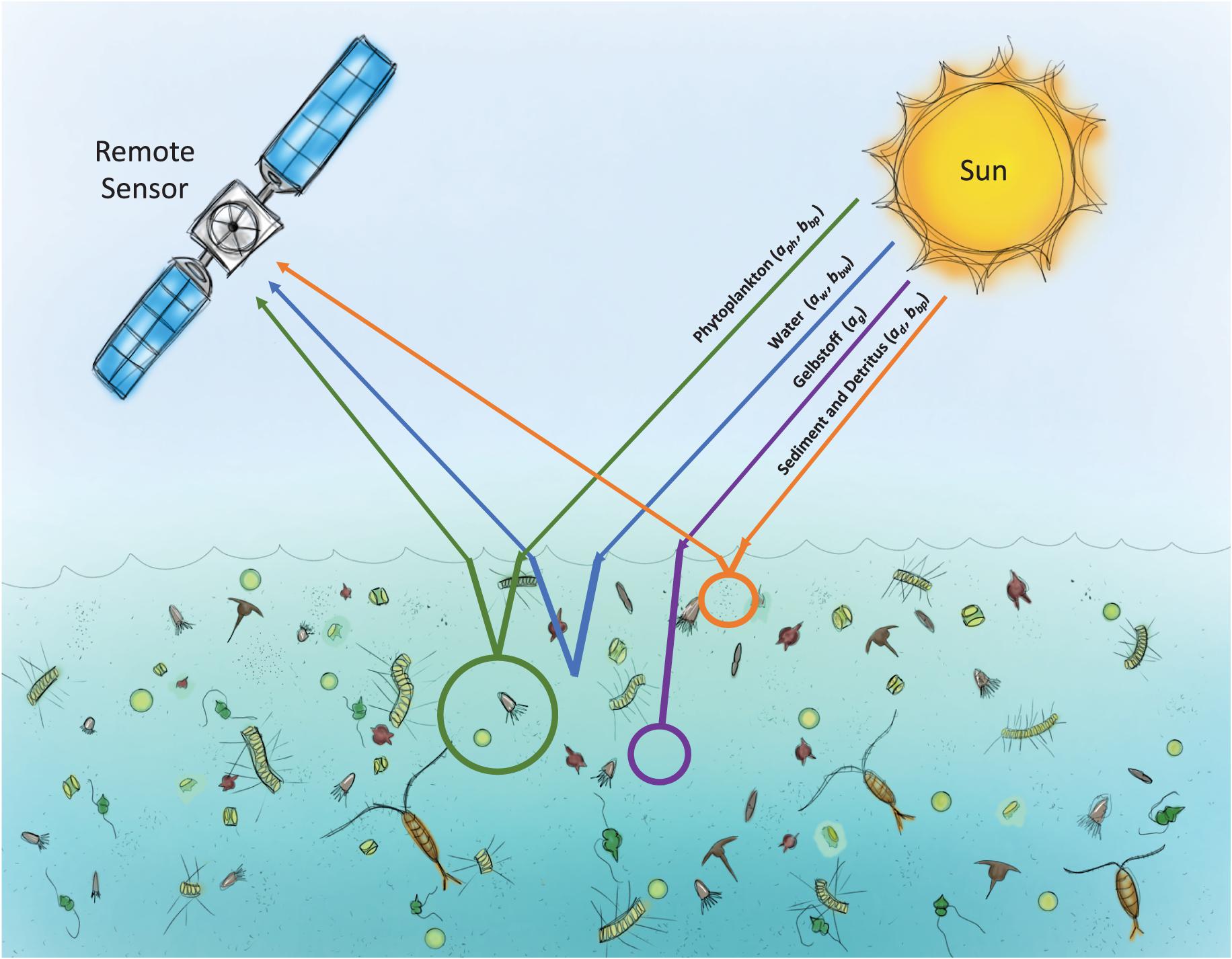
Phytoplankton can absorb and scatter light due to their pigments and their cells' structure. For example, high concentrations of phytoplankton cells usually result in high concentrations of the primary photosynthetic pigment (Chl-a). As part of photosynthesis, this pigment absorbs light (primarily in the blue region of the spectrum), leaving a larger proportion of incoming light at green wavelengths unabsorbed and more likely to be reflected, making the water look less blue and greener the higher the concentration. Beyond phytoplankton, other constituents in the oceans can affect its colour. Non-algal particles, such as sediments and coloured dissolved organic matter (CDOM), influence ocean colour and exhibit absorption and scattering properties distinct from those of phytoplankton, which vary with the sources of the sediments and dissolved matter (IOCCG, 2014).
1.1.4.2 Chlorophyll -a concentration
All green plants, cyanobacteria, and phytoplankton contain chlorophyll-a (Chl-a) as their main photosynthetic pigment (Mishra et al., 2020). Its distribution, variability, and correlation pattern with different parameters have been used to estimate biomass or primary productivity (Behrenfeld et al., 2005; Westberry et al., 2008) and to understand marine ecosystem response in the oceans (Barange et al., 2010). Marine ecological variations and biological reactions are primarily influenced by Chl-a fluctuation (Andrew et al., 2019). Chl-a concentrations indicate phytoplankton abundance and biomass in coastal and estuarine waters. Concentration of Chl-a represents the availability of phytoplankton which is mainly associated with the primary production in aquatic ecosystems (Shen et al., 2012).
1.1.5 Variability and Change in Southern Ocean phytoplankton
The Southern Ocean is the largest high-nutrient low-chlorophyll (HNLC) region over the global oceans. HNLC areas are where high levels of phytoplankton productivity and biomass that could be expected from high nutrient concentrations do not eventuate. In this region, the limited growth of phytoplankton is primarily attributable to the lack of trace minerals (i.e., silicate and iron) and light (Arrigo et al., 2008; Petrou et al., 2016). Phytoplankton in the SO, varies spatially, vertically, seasonally, and annually with the alterations of these nutrients and trace minerals (Deppeler & Davidson, 2017; Joy-Warren, 2022; Petrou et al., 2016; Prend et al., 2022).
The seasonality of the phytoplankton photosynthesis, growth, and distribution is mainly controlled by the high seasonal variation of the solar irradiance, nutrients (nitrogen, phosphorus), trace elements, sea ice, winds, and storm events (Arrigo et al., 2008; Comiso, 2010). Arrigo and van Dijken (2003); Arrigo et al. (2008) reported low levels of Chl-a are often in September, with slow increases in early spring (October). In summer, it reaches its peak concentrations and declines again to pre-bloom concentrations in March/April (Arrigo & van Dijken, 2003; Arrigo et al., 2008).
Despite this common seasonal pattern, phytoplankton biomass varies considerably among different regions of the Southern Ocean. The highest Chl-a concentrations in the SO are found in the coastal zone (CZ), and polynya systems, where favourable light conditions, stratification, and enhanced nutrient availability support elevated phytoplankton growth. In contrast, the lowest Chl-a concentrations are typically found in the open-ocean pelagic regions north of the seasonal sea ice zone, where iron limitation and weaker nutrient inputs constrain phytoplankton biomass (Arrigo et al., 2008). During the austral summer, many Antarctic coastal regions become biological hotspots, with primary productivity reaching values an order of magnitude greater than those in adjacent pelagic waters. This enhanced productivity is largely driven by increased iron inputs from the Antarctic continental shelf, sea-ice melt, and the upwelling of nutrient-rich Circumpolar Deep Water, which promote phytoplankton growth and biomass accumulation(Arrigo et al., 2008; Mann & Lazier, 2013).
At broader spatial scales, phytoplankton biomass also varies across the major Southern Ocean frontal zones and ocean basins. Using 21 years of remote sensing data Del Castillo et al. (2019) found statistically significant increases in the concentration of chlorophyll in the Subtropical Zone (STZ), Sub Antarctic Zone sectors (SAZ) as well as Permanently Open Ocean Zone (POOZ) of the Southern Ocean. These trends seem accentuated by higher chlorophyll concentrations during the austral winter due to reduced stratification, sea surface temperature, and PAR (Del Castillo et al., 2019). Ardyna et al. (2017) also reported that phytoplankton biomass is mainly organised in the southern SO at a latitudinal and regional (i.e., Indian, Pacific, and Atlantic) scale. Latitudinally, a clear gradient in the timing of bloom occurrence appears tightly linked to the seasonal cycle in irradiance, with some exceptions in specific light-limited regimes. They mentioned an extensive range of annual mean Chl-a concentration and net primary production (NPP) (>0.1 mg Chl-a m-3 /20 g Cm2y-1 to more than 2 mg Chl-a m-3 /400 g Cm2y-1 respectively) across the SO due to the iron availability (Ardyna et al., 2017).
1.2 Research Significance
Although numerous studies have provided valuable insights into phytoplankton responses to climate change, a comprehensive, multi-methodological framework integrating long-term satellite observations, advanced machine learning reconstructions, and Earth System Model projections has remained elusive for the Southern Ocean (SO). Furthermore, decadal time series are insufficient to extract climate change-driven trends in phytoplankton, as studies suggest 40+ years of data might be needed (Henson et al., 2010). Addressing these limitations, this thesis provides a unified, multi-methodological assessment of phytoplankton variability and change in the SO, advancing both observational and predictive understanding of Antarctic marine ecosystems.
Despite considerable advances in Southern Ocean research, important uncertainties remain regarding the long-term responses of phytoplankton to environmental variability and climate change. Previous studies have documented spatial and temporal changes in phytoplankton biomass, but the relative importance of different physical drivers, including temperature, mixed-layer dynamics, sea-ice variability, and large-scale climate modes, remains incompletely resolved. Furthermore, observational constraints associated with the remoteness and seasonally ice-covered nature of the Southern Ocean limit the ability to characterise long-term ecosystem variability.
Recent advances in satellite remote sensing, machine learning, and Earth System Model projections provide new opportunities to address these knowledge gaps. Long-term satellite observations enable investigation of multi-decadal phytoplankton variability, while emerging machine-learning approaches offer the potential to reconstruct spatially continuous biological fields and improve integration between observations and climate projections. However, these approaches remain underutilised in Southern Ocean research.
Addressing these knowledge gaps is important for improving understanding of Southern Ocean ecosystem responses to climate change and for reducing uncertainty in projections of future marine productivity, carbon cycling, and ecosystem functioning. The present thesis was therefore designed to combine long-term observations, physical-driver analyses, machine-learning approaches, and climate projections to improve understanding of Southern Ocean phytoplankton variability and change.
1.3 Objectives
This project aims to explore the seasonal, interannual, and multi-decadal responses and dynamics of Southern Ocean phytoplankton using satellite observations, reanalysis data, deep learning models, and climate projections, with a focus on interactions with physical drivers. To achieve this aim, the study is structured around four core objectives: 1) to quantify Southern Ocean phytoplankton variability across seasonal, interannual, and decadal timescales and examine its relationships with major physical drivers; 2) to assess the influence of sea ice variability on phytoplankton changes across the Southern Ocean; 3) to reconstruct Southern Ocean phytoplankton distributions using a deep-learning U-Net convolutional neural network; and 4) to project future phytoplankton changes by applying the trained deep-learning framework to climate projections from four CMIP6 Earth System Models under different emission scenarios.
Each of these objectives will contribute to understanding long-term changes in the Southern Ocean's ecosystem.
Project aim: Assess the variability of SO phytoplankton from seasonal to inter-annual to decadal time scales using multi-decadal records of satellite observations
Chapter 1: General introduction and literature review
Chapter 2: Spatiotemporal variability of phytoplankton from satellite observations
Characterising seasonal, interannual, and decadal variability of Southern Ocean chl-a
Assessing regional and frontal-scale patterns of phytoplankton variability
Analysing relationships with SST, MLD, PAR, and wind speed
Chapter 3: Find out the relationship between phytoplankton and sea ice.
- Assessing the relationship between satellite-derived phytoplankton trends and sea ice extent anomalies
Chapter 4: Reconstruction of phytoplankton distributions using deep learning
Developing a U-Net deep-learning framework for phytoplankton reconstruction
Evaluating model performance against satellite observations
Identifying the relative importance of environmental predictors
Chapter 5: Future projections of Southern Ocean phytoplankton under climate change
Evaluating uncertainty among selected CMIP6 Earth System Models
Applying the trained deep-learning framework to climate projections
Projecting climate-driven changes in phytoplankton and ecosystem productivity
Chapter 6: Conclusion
This chapter will summarise all results and list some limitations and future work in this regard.
1.4 Structure of the thesis
This thesis is structured into six chapters. The initial chapter offers a comprehensive introduction and scientific context to the subjects, outlining the research objectives. Chapter 2 examines the seasonal, interannual, and decadal variability of Southern Ocean phytoplankton and its relationships with major physical drivers. Chapter 3 investigates the influence of sea-ice variability on phytoplankton dynamics. Chapter 4 develops a deep-learning framework for reconstructing Southern Ocean chlorophyll-a distributions. Chapter 5 applies the trained framework to CMIP6 climate projections to assess future phytoplankton trajectories under different emission scenarios. Finally, Chapter 6 synthesises the major findings, discusses limitations, and outlines future research directions.