5 Future Trajectories of Southern Ocean Phytoplankton Under Varied Climate Change Scenarios
This chapter will be submitted to Nature Climate Change.
5.1 Abstract
Reliable projections of Southern Ocean phytoplankton are essential for understanding future climate–carbon feedbacks, yet Earth System Models (ESMs) display substantial disagreement in their chlorophyll a (Chl‑a) projections across emission scenarios. Here, we develop an observation‑constrained deep learning framework that applies a U‑Net architecture trained on satellite-derived physical–biological relationships to CMIP6 future climate simulations. The network was retrained at 1° resolution using CMIP6 physical predictors and validated against historical (1850–2014) model fields, reproducing seasonal to interannual Chl‑a variability with strong skill (ensemble r = 0.66) and minimal bias. This retraining step was undertaken to ensure consistency between the predictor fields and the climate-model environment prior to generating future projections. Applying the trained model to future physical states (2015–2100) under SSP1‑2.6, SSP2‑4.5, and SSP5‑8.5 yields substantially more coherent projections than raw CMIP6 outputs. Across all scenarios, we find consistent basin‑wide declines in Southern Ocean Chl‑a, ranging from 1-6 % decreases by 2100 under SSP5‑8.5. Spatial patterns reveal that losses are most pronounced in subantarctic and marginal‑ice‑zone bloom regions, driven primarily by warming‑induced stratification, shoaling mixed layers, reduced nutrient supply, and declining photosynthetically available radiation. These physically consistent trends contrast with the divergent Chl‑a responses in native ESM projections, highlighting the value of observation‑trained constraints for high‑latitude ecosystems. The projected declines in phytoplankton biomass imply weakened primary production, reduced carbon export efficiency, and increasing vulnerability of Southern Ocean food webs. Our results demonstrate that integrating machine‑learning‑derived empirical sensitivities with climate projections can substantially narrow uncertainty and provide more credible assessments of future ecosystem changes in the Southern Ocean.
5.2 Introduction
Reliable projections of marine phytoplankton are central to understanding future climate–carbon feedbacks and ecosystem responses. In the Southern Ocean, which accounts for approximately 50% of the global oceanic uptake of anthropogenic CO₂ through physical circulation and solubility-driven processes (DeVries et al., 2017), projections of Chlorophyll-a (Chl-a) remain among the most uncertain outputs of Earth System Models (ESMs) (Gruber et al., 2019; Hauck et al., 2023; Henley et al., 2020). Despite major advances in the Coupled Model Intercomparison Project Phase 6 (CMIP6), simulated Southern Ocean Chl-a exhibits large inter-model spread, with projections differing in both magnitude and sign across regions and emission scenarios (Buchovecky et al., 2023; Laufkötter et al., 2015; Séférian et al., 2020). For instance, under high-forcing scenarios like SSP5-8.5, some models simulate marked declines in phytoplankton biomass associated with enhanced stratification and reduced nutrient supply, while others project localized increases linked to sea-ice retreat or altered circulation pathways (Kwiatkowski et al., 2020; Ryan-Keogh et al., 2023; Tagliabue et al., 2021). This uncertainty limits confidence in assessments of biological carbon sequestration, which could weaken substantially in the region by 2100 under unmitigated warming, amplifying atmospheric CO₂ accumulation and global temperature rise (Hauck et al., 2023; Leung et al., 2015).
Much of this divergence arises from structural differences in how ESMs represent physical–biogeochemical coupling, including mixed-layer dynamics, iron limitation, light availability, and sea-ice processes (Laufkötter et al., 2015; Tagliabue et al., 2017). These inconsistencies persist even under identical forcing, highlighting the challenge of constraining Southern Ocean biological responses using process-based models alone. Such uncertainty hampers policy-relevant forecasts for carbon budgeting, krill-based ecosystems and dependent fisheries, and biodiversity under the Paris Agreement.
In parallel, satellite observations over the past two decades have provided an increasingly robust picture of surface Chl-a variability and its coupling to physical drivers such as sea surface temperature (SST), Mixed layer depth, wind forcing, and light availability (Behrenfeld et al., 2006; Martinez, Gorgues, et al., 2020). Machine learning approaches have shown strong potential for exploiting these observational records to learn empirical relationships between physical conditions and phytoplankton biomass, often outperforming traditional statistical methods in reproducing spatial patterns and temporal variability (Irrgang et al., 2021; Reichstein et al., 2019). However, most previous applications have focused on historical reconstruction or short-term prediction (Buchovecky et al., 2023), with few studies extending observation-trained models to future climate projections globally (Ryan-Keogh et al., 2025) and even fewer have addressed high-latitude oceans.
Here, we apply an observation-trained deep learning framework to constrain future Southern Ocean Chl-a projections. Building on the U-Net architecture developed in the previous chapter, which reconstructed major spatial and temporal patterns of historical Chl-a variability from satellite-derived physical predictors, we extend this framework to CMIP6 climate projections. The approach leverages empirical relationships learned from observations and applies them consistently to future physical states simulated by ESMs, providing an observation-constrained complement to process-based projections. However, as with any statistical or machine-learning framework, the reliability of projections may decrease when future environmental conditions move beyond the range represented in the training data. To reduce this risk, the model was retrained using historical CMIP6 predictor fields, thereby improving consistency between the training and projection environments.
To adapt for future projections, the U-Net was retrained at 1° resolution—matching CMIP6 outputs—using five key physical predictors: SST, sea level anomaly (SLA), mixed-layer depth (MLD), photosynthetically available radiation (PAR), and surface wind speed, all extracted from four representative ESMs (ACCESS-ESM1-5, GFDL-ESM4, IPSL-CM6A-LR, UKESM1-0-LL; Table 5.1). Historical simulations (1850–2014) served as independent validation, confirming the network's ability to replicate native ESM Chl-a (ensemble r = 0.66). Projections were then generated for 2015–2100 under SSP1-2.6, SSP2-4.5, and SSP5-8.5, with the U-Net imposing observed biological sensitivities on future physical states.
A key assumption underlying this approach is that the empirical relationships learned between surface physical conditions and phytoplankton biomass remain applicable under future climate states. However, this assumption may be challenged under strong warming scenarios, particularly SSP5-8.5, where future environmental conditions, including sea-surface temperature, sea-ice extent, stratification, and mixed-layer dynamics, may extend beyond the range represented in the training data. In such cases, the model may be required to extrapolate into novel environmental states, introducing additional uncertainty into late-century projections. Consequently, the results should be interpreted as projections conditioned on the persistence of the learned physical-biological relationships, rather than predictions that fully account for potential future ecosystem reorganization or emerging ecological processes (Behrenfeld et al., 2006; Hauck et al., 2023).
By bridging satellite observations and climate projections, this hybrid framework aims to reduce uncertainty in Southern Ocean productivity estimates, suppress physically inconsistent model behaviour, and reveal coherent, scenario-dependent Chl-a responses. More broadly, the study demonstrates how data-driven constraints can complement Earth system modelling, offering a pathway to improve projections of climate-sensitive marine ecosystems in regions where conventional models remain highly uncertain.
5.3 Data and Methods
5.3.1 Data
To capture phytoplankton dynamics, we employed two complementary datasets: (i) satellite and reanalysis products for observationally constrained model training and (ii) CMIP6 Earth System Model outputs for historical validation and future projections. Details of the observational datasets, including ecological relevance and spatiotemporal resolution, are provided in Chapter 4 (Table 4.1).
We obtained outputs from 4 CMIP6 models with three scenarios from the Earth System Grid Federation (ESGF) Nodes (Cinquini et al., 2014). For the historical period (1850–2014) and future projections, we used four CMIP6 Earth System Models (Table 5.1). Chl-a from these models was employed during historical validation, where satellite data were unavailable. Environmental drivers were consistently extracted from the same CMIP6 models to ensure compatibility. Future scenarios were examined under three Shared Socioeconomic Pathways (SSPs): SSP1-2.6 (low forcing), SSP2-4.5 (intermediate forcing), and SSP5-8.5 (high forcing) (O’Neill et al., 2016).
| Model | Ensemble Member | Ocean Component | Resolution (nominal) | Modelling Centre | Scenarios used |
|---|---|---|---|---|---|
| ACCESS-ESM1.5 | r1i1p1f1 | MOM5 | 1.0° × 1.0° | CSIRO-ARCCSS-BoM | Historical, SSP1-2.6, SSP2-4.5, SSP5-8.5 |
| GFDL-ESM4 | r1i1p1f1 | MOM6 | 1.0° × 1.0° | NOAA-GFDL | Historical, SSP1-2.6, SSP2-4.5, SSP5-8.5 |
| IPSL-CM6A-LR | r1i1p1f1 | NEMO3.6 | 1.0° × 1.0° | IPSL | Historical, SSP1-2.6, SSP2-4.5, SSP5-8.5 |
| UKESM1.0-LL | r1i1p1f2 | NEMO | 1.0° × 1.0° | MOHC | Historical, SSP1-2.6, SSP2-4.5, SSP5-8.5 |
For the historical (1850–2014) and scenario (2015–2100) periods, variables were preprocessed as described in Table 5.2.
5.3.2 CMIP6 predictors and preprocessing
Physical variables were extracted from each CMIP6 model used as predictors for Chl-a reconstruction and projection (Table 5.2): sea surface temperature (SST), mixed layer depth (MLD), sea surface height anomaly (SLA), surface downwelling shortwave radiation (converted to photosynthetically available radiation; PAR), surface wind speed, and sea-ice concentration.
All variables were converted to consistent physical units and processed following standardized procedures. SST and MLD were used directly. Sea surface height was converted to anomalies by removing the temporal mean at each grid cell. Eastward and northward wind components were combined into wind speed. Shortwave radiation was converted to PAR using a fixed conversion factor (Pinkerton & Hayward, 2021). Sea-ice concentration was not used as a predictor, but only as a spatial mask.
Because CMIP6 predictors are provided at 1° × 1° resolution, all satellite and reanalysis datasets used for training were regridded to the same resolution for a second training phase. This ensured scale consistency and enabled direct transfer of the observation-trained network to CMIP6-based projections.
In addition to changes in mean chlorophyll-a concentration, changes in the amplitude of the seasonal cycle were also evaluated. Seasonal cycle amplitude was defined as the difference between the maximum and minimum monthly climatological chlorophyll-a concentrations within a given analysis period. This metric provides an indication of changes in the strength of seasonal phytoplankton variability under future climate conditions.
| CMIP6 Variable | Description | Unit | Final Processed Form |
|---|---|---|---|
| chlos | Surface mass concentration of total phytoplankton as chlorophyll in seawater | kg m⁻³ | Converted to mg m⁻³ (chlos × 1e6) |
| mlotst | Ocean mixed layer thickness (σT criterion) | m | Used directly as Mixed Layer Depth (MLD) |
| rsds | Surface downwelling shortwave radiation | W m⁻² | Converted to PAR (Einstein m⁻² day⁻¹) using rsds × 2.10 × 10⁻⁶ (Pinkerton & Hayward, 2021) |
| zos | Sea surface height above geoid | m | Anomaly relative to the temporal mean (SLA) |
| uas, vas | Eastward and northward near-surface wind | m s⁻¹ | Combined into Wind Speed (WS): \(\sqrt{uas^{2} + vas^{2}}\) |
| tos | Sea surface temperature | °C | Used directly as SST |
| siconc | Sea-ice area fraction | % | Used as a mask; grid cells with siconc > 15% were excluded |
5.3.3 U-Net adaptation and application
The U-Net architecture, training strategy, evaluation metrics, and permutation feature importance analysis are described in detail in Chapter 4. Here, we summarize only aspects relevant to its application to CMIP6 projections.
In brief, U-Net was trained using monthly satellite-derived Chl-a (GlobColour, 2003-2010) as targets and co-located physical predictors. All predictors were standardized to zero mean and unit variance. The model was optimized using a combined loss function (80% mean squared error and 20% structural similarity index), enabling accurate reconstruction of both Chl-a magnitude and spatial structure. For this study, the U-Net was retrained at 1° resolution using the same architecture, loss function, and validation criteria as the original implementation. This retraining ensured compatibility with CMIP6 predictors and did not involve any modification of model structure or learning strategy.
The trained U-Net was then applied without further adjustment to each ESM’s future physical fields. This approach imposes empirically derived biological sensitivities from observations onto simulated physical states, providing observation-constrained projections that are directly comparable across models and scenarios.
5.3.4 Sea-ice masking
To minimize spurious Chl-a signals in ice-covered regions, sea-ice concentration from each CMIP6 model was used to apply spatial masks. Two masking strategies were evaluated: Time-varying mask where we excluded grid cells with monthly sea-ice concentration exceeding 15% and fixed largest sea-ice extent (LSIE) mask, excluding any grid cell exceeding 15% ice concentration at any point during 1850–2100. The time-varying mask was selected for all primary analyses, as it more realistically represents seasonal and interannual variability at the ice edge and preserves biologically relevant signals associated with marginal ice-zone blooms. This approach yielded higher correspondence between reconstructed and native Chl-a variability in several models (Table 5.3).
5.3.5 Historical validation
For the historical validation, a separate U-Net was retrained for each CMIP6 Earth System Model using native CMIP6 Chl-a as targets and the corresponding CMIP6 physical predictors as inputs over the 1940–1980 training period. Each model-specific network was subsequently applied to the historical physical fields (1850–2014) of the same ESM to reconstruct Chl-a,, which was compared against the model’s native Chl-a output during the pre-satellite era. This validation assesses the ability of the observation-trained network to reproduce internally consistent Chl-a variability across structurally distinct ESMs. Validation metrics included Pearson correlation coefficient (r), root-mean-square error (RMSE), mean absolute error (MAE), and mean bias.
5.3.6 Ensemble and scenario analysis
Future projections were generated for each ESM and SSP scenario for the period 2015–2100. Multi-model ensemble statistics were computed using the arithmetic mean across models, with inter-model spread quantified using the ensemble standard deviation. All analyses were performed consistently across scenarios to isolate forcing-dependent responses.
5.3.7 Trend Analysis:
To estimate long-term trends, a constant annual cycle was removed from each grid cell prior to fitting the linear regression, following the approach of Vantrepotte and Mélin (2009). While the seasonal cycle of Chl-a may vary over time (Henson et al., 2013), removing a time-varying seasonal signal through seasonal-trend decomposition (Cleveland et al., 1990) could introduce bias into the trend detection. Conversely, the use of a fixed climatological seasonal cycle implicitly assumes that seasonality remains stationary throughout the projection period. Under strong climate forcing, future changes in phytoplankton phenology and seasonal amplitude may violate this assumption and influence the estimated trends. Consequently, the reported trends should be interpreted with this limitation in mind. Linear regressions were then applied to the deseasonalized time series, and the resulting slopes were expressed as percentage change per year. For each regression, the p-value was computed, and regions with p > 0.05 were plotted with hatching. Spatially aggregated trends were calculated using the cosine of latitude as a weighting factor. To account for the heavy-tailed distribution of Chl-a, the spatial mean was used. Although spatial trend maps were derived from deseasonalized anomaly fields, the temporal trends shown in Figure 5.1 and 5.3 were calculated from the projected Chl-a changes relative to the 2015 baseline.
5.4 Results
5.4.1 Large Inter-Model Uncertainty in Raw CMIP6 Projections
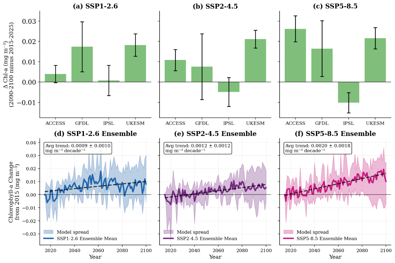
Before applying the observation-constrained U-Net framework, we first examined chlorophyll-a (Chl-a) projections directly from the four CMIP6 Earth System Models (ESMs) to quantify baseline uncertainty in Southern Ocean phytoplankton projections. CMIP6 Earth System Models exhibit extraordinary disagreement on Southern Ocean Chl-a trajectories, with individual models projecting everything from strong declines to substantial increases under identical forcing scenarios. Even when focusing on the four models assessed in this study (ACCESS-ESM1-5, GFDL-ESM4, IPSL-CM6A-LR, and UKESM1-0-LL), projections under the high-emission scenario SSP5-8.5 for the end of the century (2090–2100 compared to 2015–2025) span from a decrease of −0.006 mg m⁻³ to an increase of +0.027 mg m⁻³, equating to roughly −3% to +14% relative to current levels (Figure 5.1). Notably, despite expectations of significant warming and increased stratification, three out of four models predict a rise in surface Chl-a, with only one indicating a decline. Consequently, the multi-model average shows a slightly positive or nearly unchanged trend (+0.0020 ± 0.0018 mg m⁻³ per decade), although this masks substantial inter-model variability and contrasting responses among individual simulations. While positive Chl-a trends have also been observed in some Southern Ocean regions during the satellite era (Chapters 2 and 3), the future projections presented here should be interpreted cautiously because they depend on both the representation of future physical conditions by CMIP6 models and the assumption that the physical-biological relationships learned by the U-Net framework remain applicable under future climate states.
5.4.2 Model Validation Using Historical CMIP6 Data
To ensure that the machine learning approach (U-Net) captured the underlying physical–biological relationships rather than merely overfitting noise, we validated the reconstructed surface Chlorophyll-a (Chl-a) against historical CMIP6 data from 1850 to 2014. This validation used outputs from four Earth System Models (ACCESS-ESM1-5, GFDL-ESM4, IPSL-CM6A-LR, and UKESM1-0-LL), comparing reconstructions with native CMIP6 Chl-a simulations. Two sea ice masking strategies were tested: a time-varying mask (dynamically excluding monthly ice-covered regions) and a fixed Largest Sea Ice Extent (LSIE) mask (based on a consistent maximum ice-free domain) (Figure 5.2).
Reconstructions closely matched CMIP6 fields, reproducing both seasonal cycles and interannual variability, with only minor deviations in absolute magnitude. The mean differences between test and predicted ΔChl-a were small: 0.010 ± 0.004 mg m⁻³ (UKESM), 0.009 ± 0.005 mg m⁻³ (IPSL), 0.024 ± 0.011 mg m⁻³ (ACCESS), and 0.012 ± 0.002 mg m⁻³ (GFDL). These results indicate that the model-specific retrained U-Net framework successfully reproduced the broad driver–response relationships and Chl-a variability simulated by the corresponding CMIP6 models during the historical period. However, while the domain-averaged differences were generally small, such metrics may partially mask compensating regional biases. Furthermore, this validation demonstrates internal consistency within the CMIP6 modelling framework rather than directly validating future projections, which remain subject to uncertainties associated with climate model forcing, structural model differences, and the assumption that the learned physical–biological relationships remain applicable under future climate conditions.
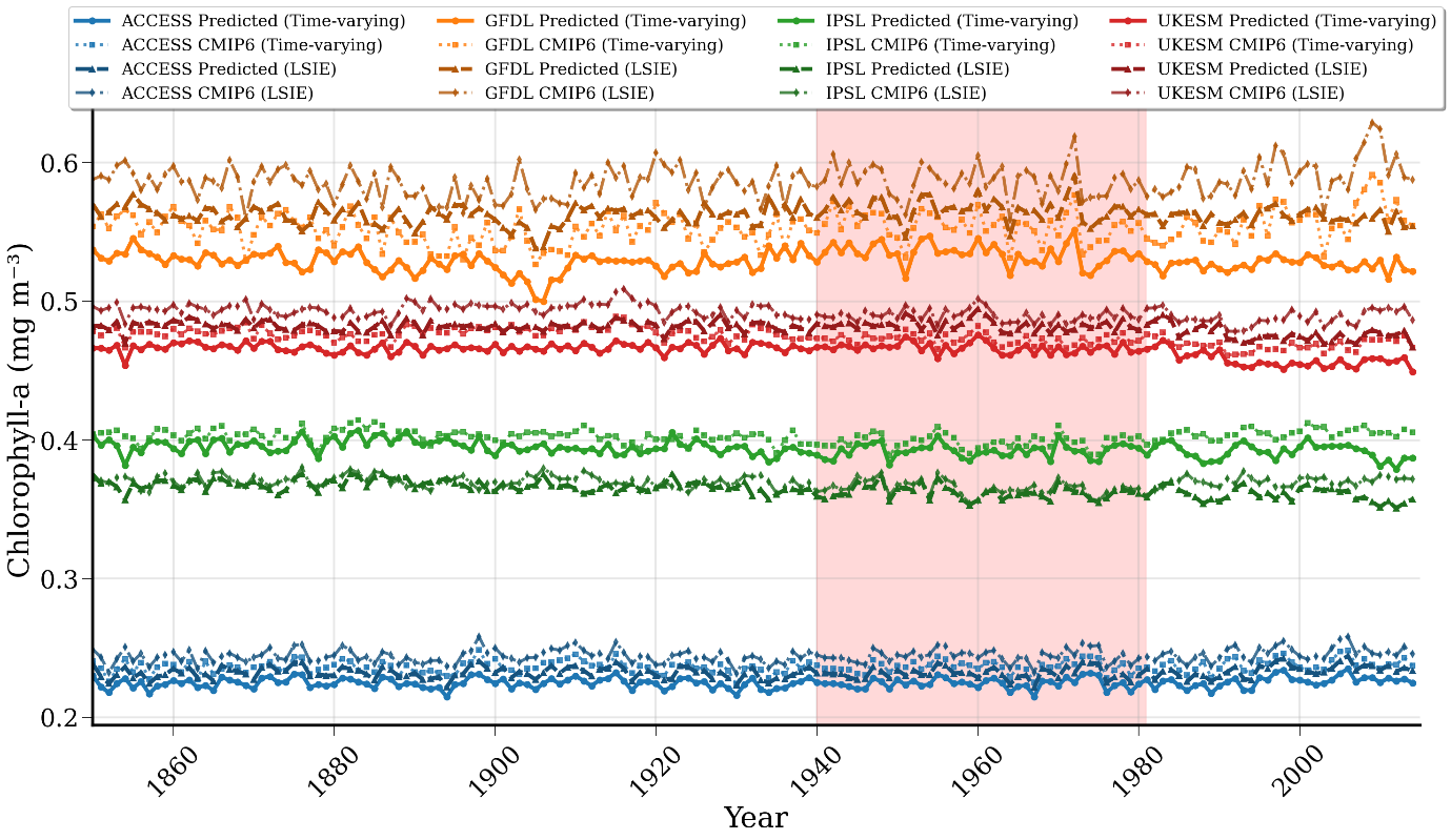
Apart from these, performance metrics also showed strong skills. For the time-varying mask, multi-model ensemble correlations averaged 0.66 (model-specific range: 0.43 for GFDL-ESM4 to 0.86 for ACCESS-ESM1-5), with root mean square errors (RMSE) averaging 0.015 mg m⁻³ (range: 0.010 mg m⁻³ for IPSL-CM6A-LR to 0.026 mg m⁻³ for GFDL-ESM4). Mean absolute errors (MAE) were 0.009–0.024 mg m⁻³, indicating minimal bias (ensemble-wide <2%). The LSIE mask had slightly lower correlations (average 0.62) but similar RMSE (0.014 mg m⁻³) (Table 5.3). The time-varying mask more effectively captured seasonal and interannual variability, with r² values exceeding 0.5 in three models, and a stronger alignment during periods of ice retreat, for instance, as seen in UKESM1-0-LL, which showed improved correlation (0.78 vs. 0.71). Bias analysis revealed a modest underestimation during bloom seasons, particularly between December and February (2–8%). Collectively, these metrics affirm the robustness of the reconstruction approach and support its application to future climate-driven projections
Table 5.3. Comprehensive validation metrics for machine learning Chlorophyll-a reconstructions. Statistical performance of reconstructed versus CMIP6 Chlorophyll-a for four Earth System Models over the validation period (1850-2014). Metrics include Pearson correlation coefficient (r), Root Mean Square Error (RMSE, mg m⁻³), Mean Absolute Error (MAE, mg m⁻³), and bias (mg m⁻³) for both time-varying sea ice mask and Largest Sea Ice Extent (LSIE) masking approaches. All models achieve correlations >0.8 and RMSE <0.01 mg m⁻³, indicating excellent reconstruction skill. A comparison between masking approaches reveals consistent performance, validating the robustness of the machine learning methodology across various sea ice treatment protocols.
| Model | Mask Type | Recons. Mean (mg m⁻³) |
CMIP6 Mean (mg m⁻³) |
MAE | RMSE | Corr. | Bias |
|---|---|---|---|---|---|---|---|
| ACCESS-ESM1-5 | Time-Varying Ice | 0.2248 | 0.2367 | 0.0119 | 0.0121 | 0.8570 | –0.0119 |
| LSIE Mask | 0.2324 | 0.2445 | 0.0121 | 0.0124 | 0.8711 | –0.0121 | |
| GFDL-ESM4 | Time-Varying Ice | 0.5294 | 0.5529 | 0.0236 | 0.0259 | 0.4280 | –0.0235 |
| LSIE Mask | 0.5628 | 0.5866 | 0.0240 | 0.0264 | 0.4295 | –0.0239 | |
| IPSL-CM6A-LR | Time-Varying Ice | 0.3939 | 0.4025 | 0.0087 | 0.0098 | 0.5696 | –0.0086 |
| LSIE Mask | 0.3648 | 0.3691 | 0.0052 | 0.0068 | 0.4912 | –0.0044 | |
| UKESM1-0-LL | Time-Varying Ice | 0.4646 | 0.4745 | 0.0099 | 0.0105 | 0.7843 | –0.0099 |
| LSIE Mask | 0.4812 | 0.4919 | 0.0107 | 0.0115 | 0.7053 | –0.0107 |
5.4.3 Observation-constrained future projections of Southern Ocean Chl-a
Having validated the reconstruction, we applied it to project Chlorophyll changes from 2015-2100 under three Shared Socioeconomic Pathways (SSP1-2.6, SSP2-4.5, and SSP5-8.5), focusing on basin-wide spatial averages south of 40°S. Using the time-varying mask, we computed yearly means and linear trends, emphasising multi-model ensemble statistics to account for inter-model variability.
Applying the U-Net to CMIP6 future physical fields yields substantially more coherent Chl-a projections than those obtained directly from the raw ESM outputs (Figure 5.3). Across all SSPs, observation-constrained projections show a consistent tendency toward declining Southern Ocean Chl-a over the 21st century. Under the low-forcing scenario (SSP1-2.6), Chl-a exhibits weak negative trends that stabilise after mid-century. The intermediate scenario (SSP2-4.5) produces sustained declines throughout the century, while the high-forcing scenario (SSP5-8.5) results in pronounced reductions, exceeding 20% relative to the late-20th-century baseline by 2100 when averaged over the basin. Compared to raw CMIP6 outputs, the spread among models is markedly reduced. While inter-model differences remain due to variations in the underlying physical drivers, the observation-constrained projections exhibit consistent trend direction and magnitude across all four ESMs.
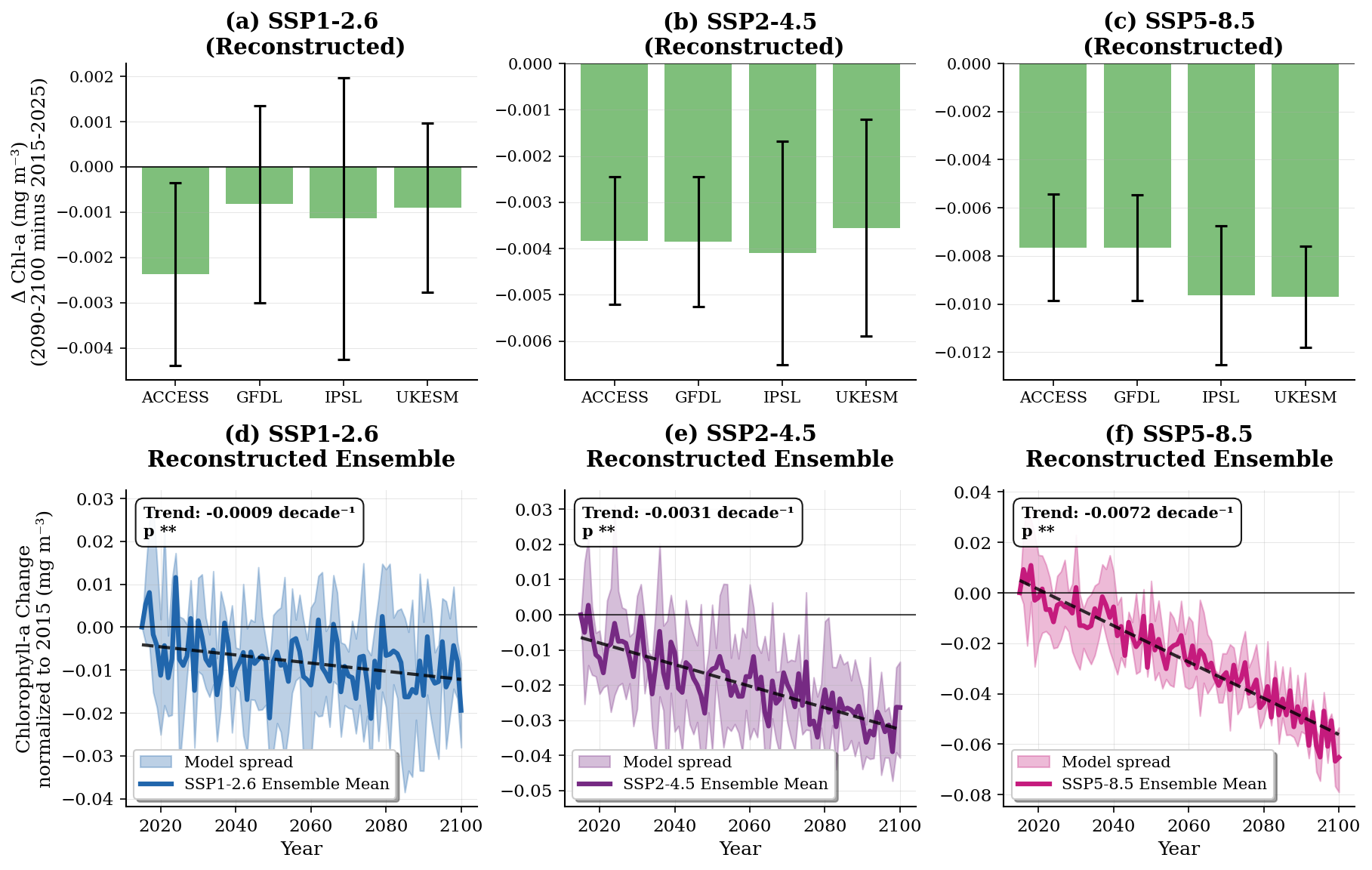
Figure 5.3: Projected Southern Ocean Chlorophyll-a trends across emission scenarios (2015-2100). Top panels (a–c) show the end-of-century (2090–2100 minus 2015–2025) changes in surface chlorophyll-a (Chl-a) concentrations for each of four Reconstructed (ACCESS, GFDL, IPSL, UKESM) under three emission scenarios (SSP1-2.6, SSP2-4.5, SSP5-8.5). Error bars represent interannual variability, highlighting the widespread and even opposing trends among reconstruction. Bottom panels, (d-f), Individual model responses (thin lines) and, multi-model ensemble means (thick lines) with uncertainty ranges (shaded areas) for three Shared Socioeconomic Pathways: SSP1-2.6 (blue), SSP2-4.5 (purple), and SSP5-8.5 (magenta). All-time series show area-weighted Southern Ocean averages (40°S-85°S) with annual mean Chlorophyll-a concentrations normalised to 2015 baseline values. Black dashed lines indicate linear trends with statistical significance assessed using least-squares regression (p < 0.05 is marked). Uncertainty ranges represent the model spread across the four-model ensemble. All scenarios exhibit statistically significant trends (p < 0.01) with aestrics (**), with higher emission pathways yielding a stronger decline in Chlorophyll, indicating a clear climate forcing of changes in Southern Ocean productivity.
In relative terms from 2015-2025 baselines, ensemble mean chlorophyll concentrations exhibit systematic declines across all scenarios, with total changes ranging from -0.85% under SSP1-2.6 (equivalent to -0.00017 mg m⁻³ decade⁻¹, 95% CI -0.0001 to -0.00024) to -5.58% under SSP5-8.5 (-0.00116 mg m⁻³ decade⁻¹, 95% CI -0.0010 to -0.0013; p<0.01 for all, based on t-test of model changes). By 2100, the end-of-century (2090-2100 mean) scenario results in a drop to 0.147-0.152 mg m⁻³ in the ensemble, representing a 1-6% reduction from the 2015 baselines (Table 5.4). Individual model projections align directionally but vary in magnitude: IPSL-CM6A-LR and UKESM1-0-LL show the steepest total declines (-6.3% and -6.2% over 2015–2100 in SSP5-8.5) (Table 5.4).
Table 5.4: Quantitative summary of relative Chlorophyll-a changes across models and scenarios. For each model-scenario combination, metrics include present-day (2015-2025) and future (2090-2100) annual means, as well as changes between the two periods. Amp. denotes the seasonal cycle amplitude (peak-to-trough range), calculated as the difference between maximum and minimum monthly climatological chlorophyll-a values.
| Model | Scenario | 2015–2025 Mean | 2090–2100 Mean | Mean Δ | 2015–2025 Amp. | 2090–2100 Amp. | Amp. Δ |
|---|---|---|---|---|---|---|---|
| ACCESS-ESM1-5 | SSP1-2.6 | 0.1609 | 0.1585 | −0.0024 | 0.1054 | 0.0931 | −0.0124 |
| GFDL-ESM4 | SSP1-2.6 | 0.1510 | 0.1502 | −0.0008 | 0.0949 | 0.0905 | −0.0044 |
| IPSL-CM6A-LR | SSP1-2.6 | 0.1497 | 0.1486 | −0.0011 | 0.0796 | 0.0723 | −0.0074 |
| UKESM1-0-LL | SSP1-2.6 | 0.1520 | 0.1511 | −0.0009 | 0.0914 | 0.0819 | −0.0094 |
| Ensemble (SSP1-2.6) | — | 0.1534 | 0.1521 | −0.0013 | 0.0928 | 0.0845 | −0.0084 |
| ACCESS-ESM1-5 | SSP2-4.5 | 0.1605 | 0.1567 | −0.0038 | 0.1042 | 0.0936 | −0.0106 |
| GFDL-ESM4 | SSP2-4.5 | 0.1520 | 0.1481 | −0.0038 | 0.0981 | 0.0876 | −0.0105 |
| IPSL-CM6A-LR | SSP2-4.5 | 0.1502 | 0.1461 | −0.0041 | 0.0811 | 0.0707 | −0.0104 |
| UKESM1-0-LL | SSP2-4.5 | 0.1540 | 0.1504 | −0.0036 | 0.0970 | 0.0854 | −0.0116 |
| Ensemble (SSP2-4.5) | — | 0.1542 | 0.1503 | −0.0038 | 0.0951 | 0.0843 | −0.0108 |
| ACCESS-ESM1-5 | SSP5-8.5 | 0.1621 | 0.1545 | −0.0077 | 0.1096 | 0.0928 | −0.0168 |
| GFDL-ESM4 | SSP5-8.5 | 0.1528 | 0.1452 | −0.0077 | 0.1030 | 0.0865 | −0.0165 |
| IPSL-CM6A-LR | SSP5-8.5 | 0.1531 | 0.1434 | −0.0096 | 0.0878 | 0.0697 | −0.0181 |
| UKESM1-0-LL | SSP5-8.5 | 0.1556 | 0.1459 | −0.0097 | 0.1004 | 0.0835 | −0.0169 |
| Ensemble (SSP5-8.5) | — | 0.1559 | 0.1473 | −0.0087 | 0.1002 | 0.0831 | −0.0171 |
5.4.4 Changes in Seasonal Cycles
Annual trends, however, mask important changes in the magnitude and amplitude of seasonal phytoplankton variability that underpin the functioning of ecosystems. To uncover these, we analysed monthly Chlorophyll cycles in near-term (2015-2025) versus end-of-century (2090-2100) periods, revealing a novel pattern of damped seasonality across SSPs and models.
Figure 5.4 presents projected changes in the seasonal cycle of Southern Ocean Chlorophyll-a (Chl-a) concentrations under three emission scenarios—SSP1-2.6, SSP2-4.5, and SSP5-8.5—by comparing present-day conditions (2015–2025) with end-of-century projections (2090–2100). Across all scenarios, the Chl-a cycle retains its characteristic austral summer peak (November–January) and autumn–winter minimum (March–May), with autumn means generally slightly lower than winter, highlighting that the baseline low-biomass period spans both seasons. Nevertheless, a consistent decline in seasonal amplitude is evident as emission intensity increases.
Quantitatively, present-day ensemble summer (DJF) means decline from 0.198 mg m⁻³ to 0.193 mg m⁻³ under SSP1-2.6 (−0.0057 mg m⁻³), from 0.201 mg m⁻³ to 0.189 mg m⁻³ under SSP2-4.5 (−0.0111 mg m⁻³), and from 0.205 mg m⁻³ to 0.181 mg m⁻³ under SSP5-8.5 (−0.0239 mg m⁻³). Correspondingly, autumn (March–May) is slightly lower than winter (June–August), changes are more minor but consistent: near-zero under SSP1-2.6 (+0.0001 mg m⁻³), −0.0029 mg m⁻³ under SSP2-4.5, and −0.0067 mg m⁻³ under SSP5-8.5. Inter-model variability remains small (0.007–0.011 mg m⁻³), confirming strong ensemble agreement. Monthly extremes reinforce this pattern: December peaks drop from 0.212 mg m⁻³ to 0.206 mg m⁻³ under SSP1-2.6, from 0.215 mg m⁻³ to 0.203 mg m⁻³ under SSP2-4.5, and from 0.220 mg m⁻³ to 0.199 mg m⁻³ under SSP5-8.5. April minima remain relatively stable under low emissions but decline to 0.1167 mg m⁻³ under SSP5-8.5.
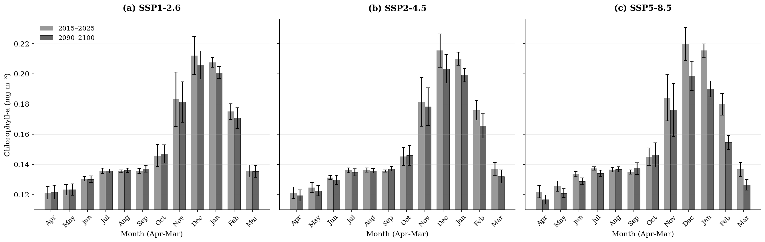
Figure 5.4:| Multi-model ensemble seasonal cycles reveal emission scenario dependency. Monthly Chlorophyll-a climatology for present-day (2015-2025, grey light) and end-of-century (2090-2100, grey dark) periods, averaged across four CMIP6 models. a, SSP1-2.6. b, SSP2-4.5. c, SSP5-8.5. Error bars indicate one standard deviation across the model ensemble. Clear scenario-dependent responses emerge: SSP1-2.6 shows minimal seasonal disruption, SSP2-4.5 exhibits moderate changes, and SSP5-8.5 demonstrates substantial seasonal restructuring. Peak amplitudes increase under higher emissions, and timing shifts become more pronounced.
5.4.5 Regional Patterns of Change
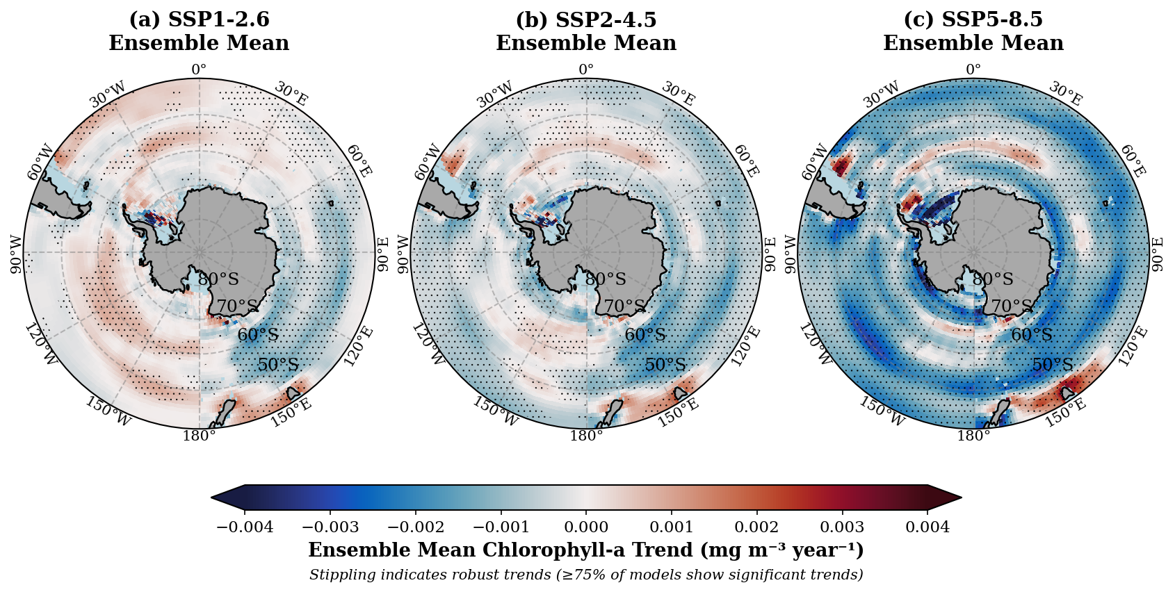
Spatial patterns of reconstructed Chlorophyll-a trends reveal strong regional heterogeneity across the Southern Ocean, with the magnitude and extent of change scaling with emission intensity (Figure 5.5). Under SSP1-2.6, declines are weak and patchy, concentrated in the Indian Ocean sector of the Southern Ocean, as indicated by limited stippling, which suggests modest model agreement. SSP2-4.5 exhibits more coherent negative trends, particularly in the Indian and Pacific and part of Atlantic sectors, where ensemble means approach −0.002 mg m⁻³ yr⁻¹ and stippling expands, signalling robust ensemble consensus. The most pronounced changes occur under SSP5-8.5, where widespread declines dominate the circumpolar region, exceeding −0.004 mg m⁻³ yr⁻¹ in subantarctic zones and marginal ice areas. The strongest declines were concentrated in these regions, whereas neighbouring regions showed weaker changes or near-neutral responses.
Quantitatively, the proportion of grid cells exhibiting positive versus negative trends, as well as the extent of statistically significant regions, further highlights the scenario dependence. Under SSP1-2.6, 43.5% of the area shows positive trends, while 56.5% indicates declines, with only 37.1% of the total area deemed significant. For SSP2-4.5, positive trends decrease to 17.4%, while negative trends increase to 82.6%, with 59.2% of the area being significant. Under SSP5-8.5, negative trends dominate 91.9% of the domain, with 87.7% of the area showing statistically significant change, reflecting robust inter-model consensus under high-emission forcing.
Localised positive anomalies (red shading) appear near coastal upwelling zones and some marginal ice regions, likely reflecting circulation-driven nutrient redistribution. However, these increases are spatially limited and overshadowed by basin-wide declines. Latitudinal gradients are evident, with subantarctic waters exhibiting the steepest reductions, while high-latitude polar regions show more minor changes, partly moderated by persistent sea ice cover. Stippling patterns confirm that robust trends emerge primarily under higher emission scenarios, with ≥75% model agreement under the SSP5-8.5 scenario.
Collectively, these spatial projections highlight that that projected chlorophyll-a changes are spatially heterogeneous across the Southern Ocean, with the largest declines concentrated in specific regions while other areas exhibit weaker changes or near-neutral responses. Such regional disparities indicate that projected chlorophyll-a responses are highly heterogeneous across the Southern Ocean, with substantial differences in the magnitude and direction of change among regions and emission scenarios.
5.4.6 Environmental Drivers of Observed Changes
Projected changes in key environmental drivers reveal strong, scenario-dependent trends that underpin the observed and reconstructed Chlorophyll-a declines in the Southern Ocean (Figure 5.6). Sea surface temperature (SST) warms consistently across scenarios, with ensemble trends ranging from +0.04 °C decade⁻¹ under SSP1-2.6 to +0.31 °C decade⁻¹ under SSP5-8.5 (p < 0.05), potential increases in upper-ocean stratification. Mixed layer depth (MLD) shoals by -0.3 to -1.9 m decade⁻¹, reducing nutrient entrainment. Wind speed strengthens slowly (+0.0 to +0.024 m s⁻¹ decade⁻¹), partially counteracting stratification by enhancing mixing, while sea level anomaly declines (-0.031 to -0.027 m decade⁻¹), signalling shifts in upwelling and circulation patterns. Photosynthetically available radiation (PAR) exhibits negligible to negative trends (up to -0.08 E m⁻² day⁻¹ in SSP5-8.5), which limits compensatory light-driven productivity in nutrient-stressed regions. These physical changes, warming, shoaling MLD, decreasing light and altered circulation, reduce nutrient availability, constraining phytoplankton growth.
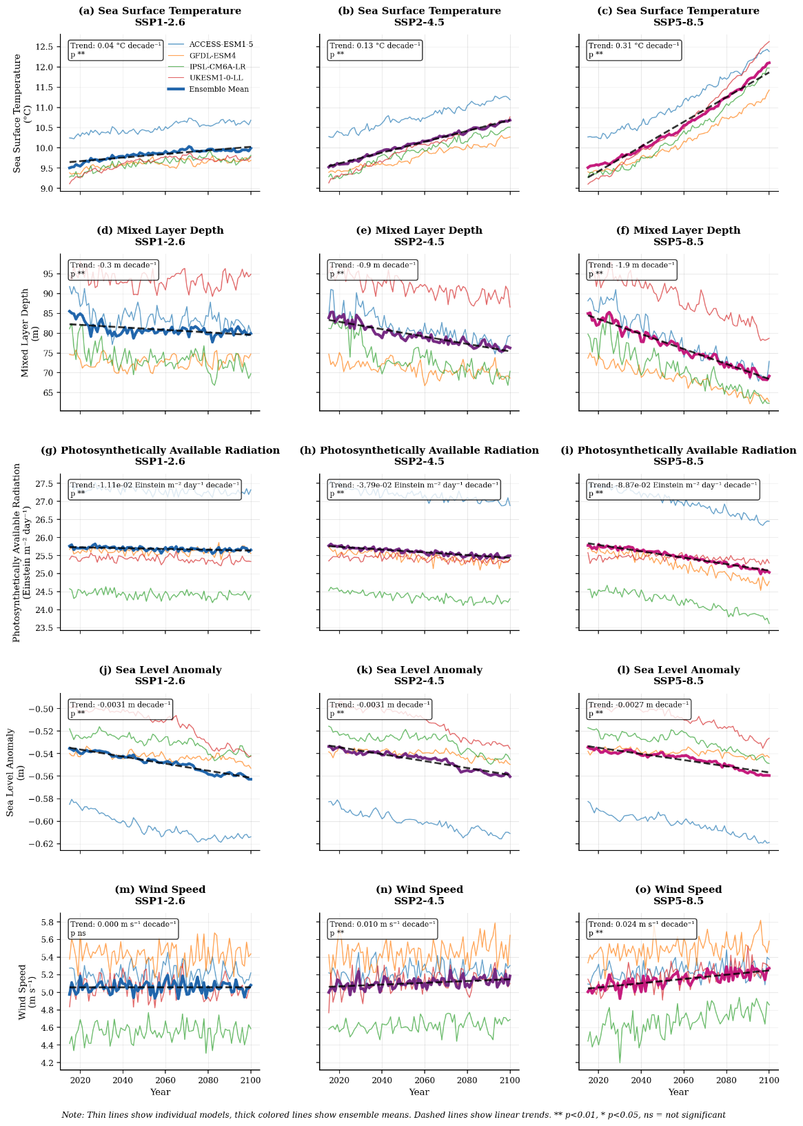
Figure 5.6: Projected changes in key environmental drivers (2015-2100). Time series of area-weighted Southern Ocean (40°S-85°S) environmental variables across three emission scenarios. a-c, Sea surface temperature. d-f, Mixed layer depth. g-i, photosynthetically available radiation. j-l, Sea level anomaly. m-o, Wind speed. Columns represent SSP1-2.6, SSP2-4.5, and SSP5-8.5 scenarios. Thin lines represent individual models; thick, coloured lines represent ensemble means. Black dashed lines indicate linear trends with significance levels marked. Trend magnitudes scale with emission scenarios, demonstrating clear climate forcing across the physical-biogeochemical system.
5.5 Discussion
5.5.1 Sources of Uncertainty in CMIP6 Chlorophyll-a Projections
The large spread in raw CMIP6 Southern Ocean chlorophyll-a (Chl-a) projections arises from multiple, interconnected sources of uncertainty, including structural differences among Earth System Models (ESMs), inconsistencies in archived diagnostic outputs, and limited observational constraints on phytoplankton responses in this data-sparse region (Laufkötter et al., 2015; Tagliabue et al., 2017). In CMIP6 models, projected Chl-a trends are primarily controlled by interactions among phytoplankton biomass, iron availability, and light limitation. However, many ESMs do not archive these limitation terms at the temporal resolution required to resolve the strong seasonality of the Southern Ocean, hindering mechanistic attribution and inter-model comparison (Laufkötter et al., 2015; Tagliabue et al., 2025).
A dominant contributor to inter-model divergence is the differing representation of physical–biogeochemical coupling. While physical forcing varies across models, the largest discrepancies stem from how biological sensitivities, such as nutrient uptake, light acclimation, and grazing, are parameterised and linked to changes in stratification, circulation, and sea-ice dynamics (Kwiatkowski et al., 2020; Séférian et al., 2020). Several CMIP6 models fail to reproduce the observed sensitivities of phytoplankton to warming-induced stratification, instead compensating for reduced nutrient supply with enhanced light or circulation-driven responses that are weakly constrained by observations (Buchovecky et al., 2023; Hauck et al., 2023).
These structural and diagnostic limitations manifest as pronounced disagreement in raw CMIP6 projections, with models differing in both the magnitude and sign of future Chl-a change under identical forcing scenarios (Figure 5.1). As uncertainty amplifies under higher emissions, relying solely on raw ESM outputs provides limited confidence in assessing future Southern Ocean productivity, motivating observation-constrained approaches that impose empirically derived biological sensitivities on future physical states.
5.5.2 Mechanisms Driving the Constrained Decline
The Southern Ocean Chl-a projections generated by the observation-constrained U-Net reveal a spatially heterogeneous response to future climate change, with the magnitude and direction of change varying among regions, scenarios, and models. While lower-emission scenarios exhibit considerable regional variability and weaker inter-model agreement, higher-emission scenarios, particularly SSP5-8.5, are characterised by more spatially coherent declines and stronger model consensus. Central to this response is sustained surface warming, which strengthens upper-ocean stratification and reduces the vertical supply of nutrients. In addition to vertical nutrient supply, Southern Ocean iron availability is influenced by several processes, including shelf-derived inputs, lateral transport, aeolian deposition, and sea-ice melt. Consequently, projected phytoplankton responses are likely to reflect the combined influence of multiple iron supply pathways rather than stratification alone (Behrenfeld et al., 2006; Henley et al., 2020). The associated shoaling of the mixed layer further suppresses macronutrient and iron entrainment in this chronically nutrient-stressed region, reinforcing biomass declines ((Ryan-Keogh et al., 2023; Tagliabue et al., 2017)).
Although wind speeds increase modestly in future projections, these changes occur alongside substantial warming and declining nutrient availability across much of the Southern Ocean. Photosynthetically available radiation also decreases in several regions under the higher-emission scenarios. Together, these environmental changes coincide with reductions in chlorophyll-a concentrations and seasonal cycle amplitude. Similar changes in Southern Ocean phytoplankton seasonality and phenology have been reported in previous studies (e.g., (Pinkerton et al., 2021; Soppa, 2015; Thomalla et al., 2023)), although phenological metrics were not explicitly evaluated in the present study.
Spatially, the strongest declines occur in subantarctic waters and marginal ice zones, where phytoplankton growth is particularly sensitive to iron limitation induced by stratification (Ryan-Keogh et al., 2023). Not all regions exhibited declining chlorophyll-a concentrations. While localized increases persist parts of the Atlantic sector and in several shelf-influenced regions, including areas downstream of Tasmania, South America, and the Antarctic Peninsula. These regions may be influenced by processes not directly represented by broad-scale nutrient limitation arguments, including frontal dynamics, shelf-bathymetry interactions, and enhanced iron supply from continental margins . By enforcing empirically derived biological sensitivities, the U-Net avoids compensatory responses common in raw ESMs—such as unrealistically enhanced productivity under warming—yielding projections that align more closely with observed historical changes and emerging BGC-Argo evidence of declining Southern Ocean productivity (Kwiatkowski et al., 2020; Séférian et al., 2020).
5.5.3 Ecosystem and Carbon-Cycle Implications
The observation-constrained decline in Southern Ocean Chl-a projected in this study has important implications for marine ecosystems and the global carbon cycle, particularly under high-emission pathways. As Chl-a is a first-order indicator of phytoplankton biomass, sustained reductions in surface concentrations imply a weakening of primary producer stocks that form the base of the Southern Ocean food web (Deppeler & Davidson, 2017). This region supports a highly efficient but vulnerable ecosystem dominated by krill, which in turn sustains higher trophic levels including fish, seabirds, seals, and migratory whales (Ducklow et al., 2013; Henley et al., 2020; Kawaguchi et al., 2023; Rogers et al., 2020). Even modest, spatially coherent declines in phytoplankton biomass can therefore propagate disproportionately through the trophic system, especially in subantarctic and marginal ice-zone regions where productivity is tightly constrained by nutrient and iron availability.
From a biogeochemical perspective, reduced phytoplankton biomass is expected to weaken the efficiency of the biological carbon pump by lowering the production of organic matter available for export to the ocean interior (Moline et al., 2004). The Southern Ocean plays a disproportionate role in global carbon sequestration, and changes in surface biomass have been shown to exert strong control on air–sea CO₂ fluxes and export production (Frolicher et al., 2015; Hauck et al., 2023). Observation-constrained declines in chlorophyll-a therefore imply a reduced capacity of this region to buffer anthropogenic CO₂ emissions, reinforcing positive climate feedbacks under continued warming (Bourgeois et al., 2022; Gloege et al., 2021).
Importantly, the ecological and carbon-cycle consequences inferred here differ qualitatively from those suggested by many raw CMIP6 projections, which often simulate stable or increasing phytoplankton biomass. By enforcing observed sensitivities between physical drivers and chlorophyll-a, the U-Net-based projections indicate a more vulnerable Southern Ocean ecosystem than implied by unconstrained ESMs. If realised, these regional declines could have important consequences for Southern Ocean food webs, carbon export efficiency, and biogeochemical cycling, particularly under high-emission scenarios. This highlights the risk of relying on raw model outputs for impact assessments and underscores the importance of observation-informed approaches for evaluating future ecosystem functioning and climate feedbacks in high-latitude oceans.
5.5.4 Limitations and Future Directions
While the observation-constrained framework developed in this study substantially reduces uncertainty in Southern Ocean Chl-a projections, several limitations should be acknowledged. First, the U-Net was trained on satellite-derived surface Chl-a, which primarily reflects near-surface phytoplankton biomass and does not explicitly resolve subsurface chlorophyll maxima that are prevalent south of the Polar Front. As a result, projected changes in vertically integrated biomass and export production can only be inferred indirectly. Future extensions that incorporate depth-resolved observational constraints from BGC-Argo floats or data-assimilative reconstructions would enable more comprehensive assessments of ecosystem and carbon cycle responses.
Second, although the U-Net imposes empirically derived biological sensitivities on future physical states, it remains dependent on the quality and representativeness of the training data. Satellite chlorophyll retrievals in the Southern Ocean are affected by persistent cloud cover, low solar angles, and seasonal sea-ice contamination, which introduce observational uncertainties that may propagate into the learned relationships. Expanding training datasets with emerging multi-sensor products and improved bio-optical algorithms will be critical for further strengthening observational constraints in high-latitude regions.
Third, the framework assumes that present-day empirical relationships between physical drivers and chlorophyll-a remain valid under future climate states. While this assumption is supported by the physically interpretable responses identified here, it may be challenged if novel ecosystem regimes emerge under extreme warming or altered nutrient stoichiometry. Incorporating adaptive or hybrid approaches that combine machine learning with mechanistic constraints from process-based models represents a promising avenue for addressing potential non-stationarity.
Finally, this study focused on a limited subset of CMIP6 models and a small set of key physical predictors. Extending the approach to a broader ensemble, including additional climate scenarios and expanded predictor sets—such as micronutrient availability, ecosystem structure, and grazing pressure—would provide a more comprehensive assessment of future Southern Ocean productivity. Together, these developments point toward a next generation of observation-informed projections that can more robustly inform ecosystem management, carbon-cycle assessments, and climate mitigation strategies.
5.6 Conclusions
Using an observation-trained U-Net applied to CMIP6 physical fields, we provide the first empirically constrained projections of Southern Ocean phytoplankton biomass for the period up to 2100. Projected chlorophyll-a responses exhibit substantial regional and scenario-dependent variability, with lower-emission scenarios characterised by greater spatial heterogeneity and weaker inter-model agreement, while higher-emission scenarios show more widespread declines and stronger model consensus. Ensemble-mean chlorophyll-a reductions range from approximately 0.9–6% by 2100 (SSP1-2.6 to SSP5-8.5), accompanied by marked reductions in seasonal cycle amplitude (>22% under SSP5-8.5) and geographically heterogeneous spatial responses. These projected changes are associated with concurrent changes in environmental conditions, including warming, mixed-layer dynamics, nutrient-related variables, and photosynthetically available radiation. Collectively, the results suggest increasing pressure on Southern Ocean phytoplankton communities under stronger warming scenarios, with the magnitude of projected change scaling broadly with future greenhouse gas emissions. In contrast, lower-emission pathways are associated with smaller and less spatially coherent changes in chlorophyll-a.