3 Sea Ice Extent Anomalies Impact Interannual Variability of Phytoplankton Chlorophyll-a in Southern Ocean Frontal Zones
This chapter has been submitted to Geographical Research Letters, and is currently under review as Golder, M. R., & Antoine, D. (2025). Chapter 3 Sea Ice Extent Anomalies Impact Interannual Variability of Phytoplankton Chlorophyll-a in Southern Ocean Frontal Zones. Geographical Research Letters
3.1 Abstract
The influence of sea-ice variability on Southern Ocean productivity across major oceanic frontal zones remains poorly quantified. Using 26 years (1998–2023) of satellite data, we quantified how sea-ice extent anomalies (SIEA) are associated with phytoplankton Chlorophyll-a (Chl-a) across three frontal zones. Summer (February) SIE declined at a rate of 2.4 × 10⁴ km² yr⁻¹, approximately 5× faster than winter (September) in relative terms (−1.1%/yr vs. −0.2%/yr), indicating a growing seasonal asymmetry. Lagged correlations show that positive SIEA precede enhanced Chl-a (36–40%, p < 0.01) in coastal and Southern Boundary zones. Post-2015, SIEA declined by 8.1% (from 11.88 to 10.91 million km², with -17.4% anomaly in 2023), and Chl-a declined from 2.6 to 6.7% across zones, indicating a recent period of low sea -ice and lower mean Chl-a in ice-proximal regions. Unlike basin-wide studies, this frontal-scale analysis resolves regionally variable lagged associations between sea-ice anomalies and phytoplankton biomass, consistent with possible sea-ice-associated preconditioning mechanisms rather than direct mechanistic attribution.
3.2 Introduction
The Southern Ocean is undergoing significant changes in phytoplankton dynamics due to climate variability, yet these changes are spatially heterogeneous and remain uncertain (Deppeler & Davidson, 2017; Montes-Hugo et al., 2009). Satellite records show high phytoplankton biomass along the Antarctic coast, in the Ross Sea, and the western Antarctic Peninsula, regulated by sea ice, sea surface temperature (SST), mixed layer depth (MLD), winds, and light availability (A. Hayward et al., 2025; Prend et al., 2019). Despite advances in characterizing these drivers, the specific mechanisms by which sea ice influences phytoplankton productivity in the Antarctic ice zone, where blooms are a prominent feature; remain underexplored (Horvat et al., 2022; Mcclish & Bushinsky, 2023; Taylor et al., 2013).
Sea ice has multiple influences on phytoplankton by modulating key environmental conditions. Melting ice forms a shallow, stable surface layer that retains phytoplankton in the euphotic zone, while also releasing ice algae and iron that stimulate growth (Arrigo et al., 2008; Lester et al., 2021; Smith & Comiso, 2008). This process contributes substantially to Southern Ocean primary production and exhibits strong seasonal variability e (Ardyna et al., 2017; Taylor et al., 2013). In addition, sea-ice formation can contribute to winter brine rejection and convective deepening, which may entrain iron-rich waters from below the ferricline into the surface layer before the following bloom season. These pathways indicate that sea ice can influence phytoplankton through both melt-season processes and winter preconditioning, making sea ice a central yet complex driver of phytoplankton variability (Llort et al., 2015; Meiners et al., 2025; Tagliabue et al., 2014).
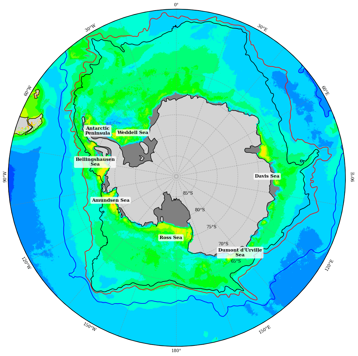
In recent decades, Antarctic sea ice extent has shown marked temporal variability, with a long-term increase followed by an abrupt decline in post 2015 (Purich & Doddridge, 2023). This shift, with record-low extents in 2023 (Hobbs et al., 2024), has potential implications for marine ecosystems and carbon cycling, although the available evidence does not by itself demonstrate a regime change. Building on this context, we hypothesize that positive sea-ice extent anomalies (SIEA) enhance the following year Chlorophyll-a (Chl-a), with stronger coupling in coastal and Southern Boundary zones, weakening toward the Polar Front. Despite progress in understanding sea ice-phytoplankton interactions, the influence of SIEA on phytoplankton remains poorly constrained at the scale of Southern Ocean frontal zones. Most prior studies emphasize basin-wide or seasonal dynamics, often overlooking spatial variability across fronts, which is critical for resolving regional ecological responses. To address this gap, we examine the relationship between SIEA and Chl-a anomalies over 1998–2023 across three key regions (Figure. 1): (1) Southern Boundary to the Antarctic coast, (2) Southern Antarctic Circumpolar Current Front (SACCF) to the Southern Boundary, and (3) Polar Front to the SACCF.
3.3 Data and Methods
We used satellite-derived datasets to assess Chl-a and sea ice dynamics over 1998–2023. For Chl-a, we used daily non-interpolated Level 3 Mapped 4×4-km resolution Global Ocean Colour data from the Copernicus Marine Environment Monitoring Service (CMEMS, https://marine.copernicus.eu/). We aggregated the daily data into monthly composites to improve the temporal and spatial coverage. By utilising this merged data product, we overcome the limitations of single-satellite datasets and gain comprehensive insight into 26 years of phytoplankton variability in the Southern Ocean.
The three frontal zones are, from south to north: the Southern Boundary Front (SB), the Southern Antarctic Circumpolar Current Front (SACCF), and the Polar Front (PF) (Figure 3.1). The mean positions of these fronts were obtained from satellite altimetry-derived ocean dynamic topography, as described by Park and Durand (2019); Park et al. (2019). For detailed information on Chl-a averages across these frontal regions, please refer to (Golder & Antoine, 2025).
For sea ice, we used Southern Hemisphere Version 3 monthly sea ice extent indices from the National Snow and Ice Data Center (NSIDC, 1979–present), restricting analysis to 1998–2023. Monthly anomalies were calculated by subtracting the climatological mean from each monthly value. Annual Chl-a and SIE anomaly series were then calculated as the mean of the 12 monthly anomalies within each calendar year; these are therefore annual means of monthly anomalies rather than anomalies of annual means. Seasonal trends (February and September) were assessed using NSIDC sea ice concentration data (Fetterer et al., 2017). Anomalies were normalized via z-score transformation, z = (x - μ) / σ, where x is observed extent, μ is the 1998–2023 mean, and σ is the standard deviation, with regimes classified as High Ice (z > 0.5), Low Ice (z < -0.5), and Normal Ice (-0.5 ≤ z ≤ 0.5) based on climatological variability. The ±0.5 threshold was selected to separate moderately positive and negative sea-ice years while retaining sufficient sample sizes in each category; sensitivity to alternative thresholds should be tested in future analyses.
3.4 Results and Discussion
3.4.1 Seasonal and interannual variability of Antarctic Sea ice extent
The annual Antarctic Sea ice extent (SIE) time series from 1998 to 2023 shows pronounced seasonality and substantial interannual variability (Figure 3.2C). Seasonal decomposition highlights faster summer (February) declines relative to winter (September) with linear trends of 24,263 km² yr⁻¹ (p = 0.020) and September at 35,178 km² yr⁻¹ (p = 0.023), respectively. In absolute terms, winter decline is ~1.45 times faster; however, when expressed as a relative change (from baselines of average summer and winter SIE respectively), the summer decline is ~5 times faster (−1.1%/yr vs. −0.2%/yr), or −11.1%/decade vs. −2.1%/decade. This asymmetric loss agrees with recent reports that Antarctic summer sea-ice retreat is accelerating (Swathi et al., 2025; Turner et al., 2022). Summer reduction is amplified by enhanced ocean–atmosphere heat fluxes and ice–albedo feedbacks (Parkinson & Cavalieri, 2012), whereas winter growth remains more strongly controlled by thermodynamic freezing and wind-driven redistribution (Frew et al., 2019). These findings indicate that summer ice dynamics are increasingly vulnerable to climate forcing.
Trend maps for February and September Sea ice concentration (SIC) reveal pronounced regional heterogeneity across the Southern Ocean (Figure 3.2A, B). During summer (February), strong negative trends (ice loss) are observed in the Ross Sea and the northern part of the Weddell Sea. In contrast, the Amundsen and Bellingshausen Seas, along with the southern Weddell Sea, exhibit muted or mixed signals. In winter (September), the most evident trends occur along frontal zones such as the Southern Boundary (SB) to the Southern Antarctic Circumpolar Current Front (SACCF), with predominantly negative trends in the Atlantic sector. The Indian and Pacific sectors exhibit mixed trends, and coastal Antarctic areas generally show near-zero changes. This spatial variability indicates that seasonal sea-ice advance and retreat differ substantially among sectors, particularly during the transition from winter maximum extent toward spring retreat and summer minimum conditions (Holland, 2014; Stammerjohn et al., 2012; Zhao et al., 2023).
The observed seasonal asymmetry and regional contrasts indicate substantial spatial and seasonal heterogeneity in Antarctic sea-ice change, rather than providing direct evidence for a regime shift or increasing instability. Because phytoplankton blooms typically initiate soon after sea-ice retreat, such shifts in the timing and magnitude of summer ice loss are expected to influence regional Chl-a variability and primary production. The following sections therefore examine how evolving sea-ice conditions modulate Chl-a anomalies and ecosystem responses across key Southern Ocean frontal zones. This change has also significant implications for both climate physics and biogeochemical processes (Boyd et al., 2024; Hobbs et al., 2024). Understanding these impacts is crucial for enhancing Earth system models, informing policy (e.g., fisheries limits), and understanding their effects on the carbon cycle.
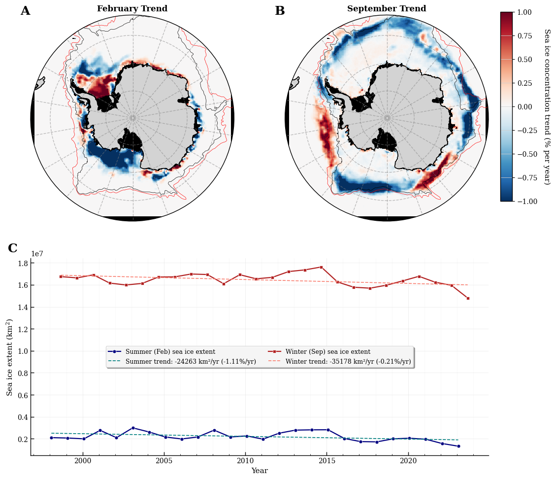
Figure 3.2: Interannual changes of summer and winter sea ice extent and spatial distribution of their long-term trends (1998–2023). Panels A and B display spatial patterns of sea ice concentration trends for the same months, expressed as percent change per year. February was selected to represent the approximate austral summer sea-ice minimum, while September was selected to represent the approximate winter sea-ice maximum. Blue shading indicates declines, red indicates increases, and frontal positions of the Southern Boundary (SB) and Southern Antarctic Circumpolar Current Front (SACCF) are overlaid for reference. Panel C shows time series of area-weighted sea ice extent for austral summer (February) and winter (September), derived from NSIDC sea ice concentration fields. Annual values were computed by summing grid-cell concentrations over the Antarctic domain, and linear trends were fitted using least-squares regression.
3.4.2 Relationship between sea ice extent anomalies and Chlorophyll-a
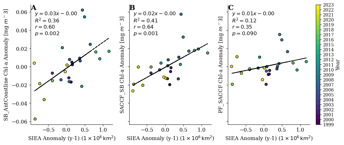
Building on the observed seasonal and regional changes in sea ice, we next examined the link between annual SIEA and annual Chl-a anomalies across three SO frontal regions (Figure 3.3A-C). In the SB_AntCoastline region, Chl-a anomalies show a strong positive association with the 1-year-lagged SIEA (r = 0.60, p = 0.002, R² = 0.36). A similar relationship is evident in the SACCF_SB region (r = 0.64, p = 0.001, R² = 0.41). In contrast, the PF_SACCF region exhibits weaker, non-significant coupling (r = 0.35, p = 0.090, R² = 0.12). Regression slopes suggest that a +1 × 10⁶ km² anomaly in SIE is followed by ~0.02–0.03 mg m⁻³ increase in annual Chl-a anomalies in the subsequent year for the coastal and Southern Boundary sectors.
The positive, lagged relationships in the coastal and southern frontal zones suggest that sea ice may precondition the upper ocean for enhanced phytoplankton growth. These results are consistent with mechanisms such as melt-related stratification, iron release from sea ice, and possible ice-algal seeding (Ardyna et al., 2017; Arrigo et al., 2008). However, the lagged relationship may also reflect winter preconditioning during sea-ice formation, where brine rejection promotes convective deepening and entrains iron-rich waters from below the ferricline, as highlighted by Giddy et al. (2023) in the northeast Weddell Sea. The 1-year lag should therefore be interpreted as evidence of sea-ice-associated preconditioning rather than direct proof of meltwater iron supply alone. In contrast, the weaker coupling in the northern PF–SACCF region likely reflects dominance of open-ocean processes such as deep mixing and upwelling (Llort et al., 2015; Tagliabue et al., 2014). Together, these results indicate that the influence of sea ice on phytoplankton productivity is strongest near the Antarctic coast and diminishes toward the open ocean frontal zones.
3.4.3 Temporal co-variability and post-2015 decline
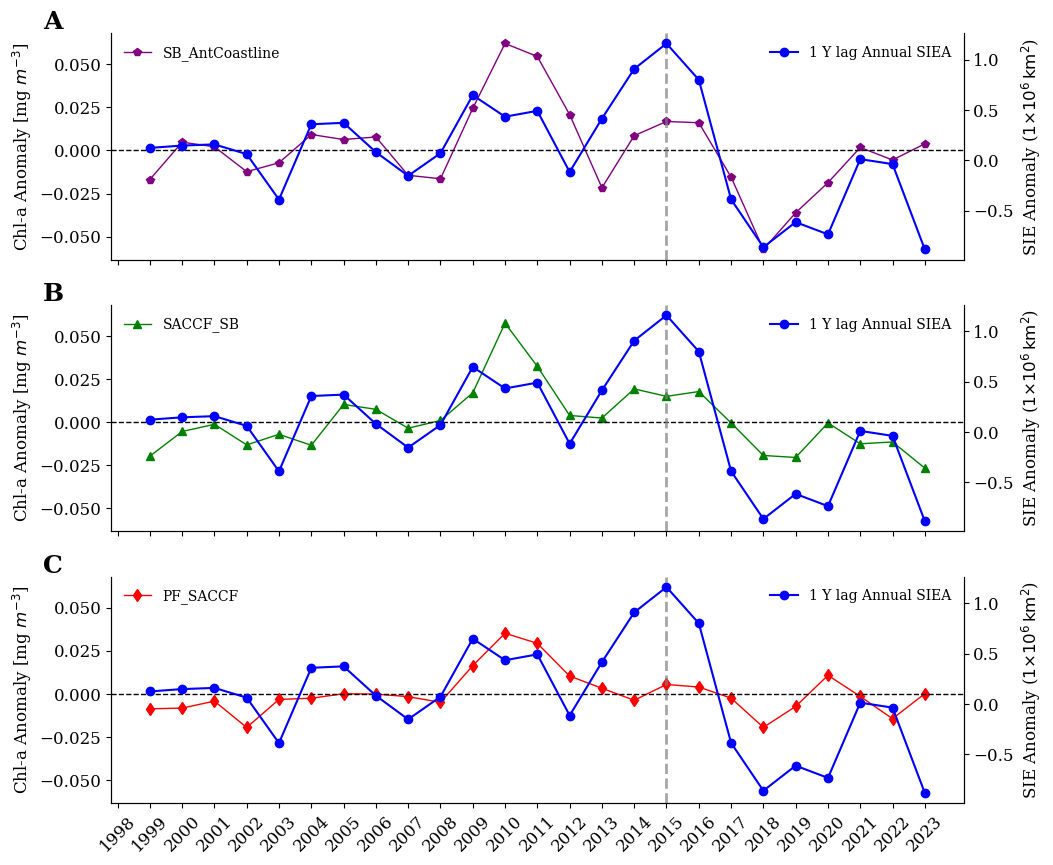
Figure 3.4A-C reveals strong temporal co-variability between annual lagged SIEA and Chl-a anomalies across the SO, with the tightest coupling in the SB–Antarctic Coastline and SACCF–SB regions (r = 0.60–0.64, p < 0.01). During 1998–2015, positive SIEA coincided with elevated Chl-a anomalies of +5–7 % relative to climatology. These patterns indicate temporal association between sea-ice and Chl-a variability; potential mechanisms are considered cautiously because stratification, iron supply, grazing pressure, and other biological controls were not directly measured here (Boyd et al., 2012; Smith & Nelson, 1985).
Post-2015, both sea-ice and phytoplankton conditions declined in the ice-proximal regions. Mean Antarctic SIE decreased by ≈ 8.15 % (from 11.87 to 10.90 million km²), reaching an extreme −17.37 % anomaly in 2023. Concurrently, mean Chl-a concentrations declined by −6.73 % in the SB–Antarctic Coastline region (0.299 → 0.279 mg m⁻³), −5.5 % in the SACCF–SB (0.239 → 0.226 mg m⁻³), and −2.6 % in the PF–SACCF zone (0.207 → 0.201 mg m⁻³). These synchronous reductions coincide with the record 2016–2017 sea-ice collapse (Meehl et al., 2019; Turner et al., 2017), but the present analysis cannot determine whether sea-ice loss directly caused the Chl-a decline. Possible contributing mechanisms include reduced melt-season stratification, altered iron supply, changes in grazing pressure, and shifts in phytoplankton community structure, all of which require additional observations to evaluate (Lester et al., 2021; Morán et al., 2010).
Regional contrasts further reveal local modulation. The PF–SACCF zone shows weaker coupling (r = 0.35, p ≈ 0.09), suggesting that sea-ice variability is less consistently associated with Chl-a variability north of the SACCF (Rintoul, 2018). Correlation changes between pre- and post-2015 periods (e.g., SACCF–SB: r ≈ 0.27 → 0.6) support a better link between sea-ice anomalies and productivity as ice retreat accelerates. The consistent one-year lag indicates a system-memory effect, possibly tied to nutrient retention or iron availability from prior melt seasons (Ardyna et al., 2017; Lannuzel et al., 2016).
Together, the ~8.15 % loss of Antarctic SIE and ~6 % decline in ice-proximal Chl-a in post-2015 indicate a recent period of reduced mean phytoplankton biomass. These patterns highlight the need for sustained satellite and biogeochemical observations to track the evolving sea-ice–ecosystem linkage, but they should not be interpreted as proof of a new baseline productivity regime without longer records and process-based evidence.
3.4.4 Sea Ice Regime Dependent Chl-a responses
Building on the observed post-2015 decline in both SIE and Chl-a, we examined how phytoplankton biomass varies under distinct sea-ice regimes across Southern Ocean frontal zones (Figure 3.5). The standardized SIE anomaly (SIEA; Figure 3.5A) identified three regimes: High-Ice (> +0.5 SD), Normal-Ice (± 0.5 SD), and Low-Ice (< −0.5 SD). High-Ice conditions occurred in 9 years (2003–2004, 2008-2010, 2012-2015), Normal-Ice in 10 years, and Low-Ice in 7 years (mostly after 2016), indicating an increasing dominance of reduced-ice conditions in the past decade.
Mean Chl-a concentrations varied across these regimes but differences were not statistically significant at the p < 0.05 level. However, consistent regional tendencies emerged (one-way ANOVA: PF_SACCF p = 0.069; SACCF_SB p = 0.077; SB_AntCoastline p = 0.115), suggesting near-significant sensitivity of phytoplankton biomass to sea-ice conditions. In the southernmost SB–Antarctic Coastline zone, High-Ice years yielded the highest mean Chl-a (0.31 ± 0.03 mg m⁻³), corresponding to an increase of +3.7 ± 3.2 % relative to climatology, whereas Normal- and Low-Ice regimes averaged 0.29 ± 0.02 mg m⁻³ (0.4 ± 2.5 %) and 0.27 ± 0.02 mg m⁻³ (–5.2 ± 3.9 %), respectively. The intermediate SACCF–SB region showed a similar but weaker pattern, with High-Ice years averaging 0.25 ± 0.02 mg m⁻³ (+4.5 ± 2.7 %) and Low-Ice years 0.22 ± 0.02 mg m⁻³ (–4.5 ± 4.1 %). Similarly, the northern PF–SACCF zone displayed a similar relationship, where High-Ice regimes corresponded to high Chl-a (0.21 ± 0.01 mg m⁻³, 3.1 ± 3.8 %), while Normal- and Low-Ice regimes exhibited (+0.1 ± 2.9 % and -4.1 ± 3.5 %, respectively) (Figure 3.5B).
These patterns mean Chl-a responses to sea-ice variability are regionally coherent but should be interpreted cautiously because the differences among regimes are not statistically significant at p< 0.05. In ice-proximal regions (SB–AntCoastline, SACCF–SB), extensive winter ice likely preconditions the upper ocean through freshwater stratification and the release of melt-derived iron, supporting later and more sustained blooms (Lannuzel et al., 2016). In contrast, low-ice years produce deeper mixed layers and weaker stratification, limiting light and nutrient retention, and reducing bloom magnitude (Llort et al., 2015; Tagliabue et al., 2014). The PF–SACCF zone, dominated by upwelling and eddy mixing, exhibits the same behaviour—where reduced ice and enhanced open-water exposure favour earlier, shorter blooms (Carranza & Gille, 2015; Thomalla et al., 2023).
A notable exception occurred in 2023, when record-low Antarctic sea ice (−16.7% SIEA) (Hobbs et al., 2024; Purich & Doddridge, 2023) coincided with an anomalously high Chl-a (+1.5% Southern Ocean mean). This single-year response may reflect increased open-water light exposure, regional redistribution of productivity, or other unmeasured physical and biological factors, but these explanations remain hypotheses because light availability and mixed-layer conditions were not directly analysed here (Boyd et al., 2016; Alexander Hayward et al., 2025; Ryan-Keogh et al., 2023).
Overall, these results show that sea-ice regimes are associated with differences in mean Chl-a across Southern Ocean frontal zones. High-Ice years generally correspond to higher mean Chl-a, whereas Low-Ice years correspond to lower mean Chl-a, with regional variability and without statistically significant differences at p < 0.05. Therefore, conclusions about earlier, later, shorter, or longer blooms are not supported by the present regime analysis and would require dedicated phenological metrics. The observed mean biomass differences nevertheless suggest that future reductions in Antarctic sea ice may affect phytoplankton biomass and could have implications for carbon cycling and food-web dynamics (Arrigo, 2014; Rogers et al., 2020; Steiner et al., 2021).
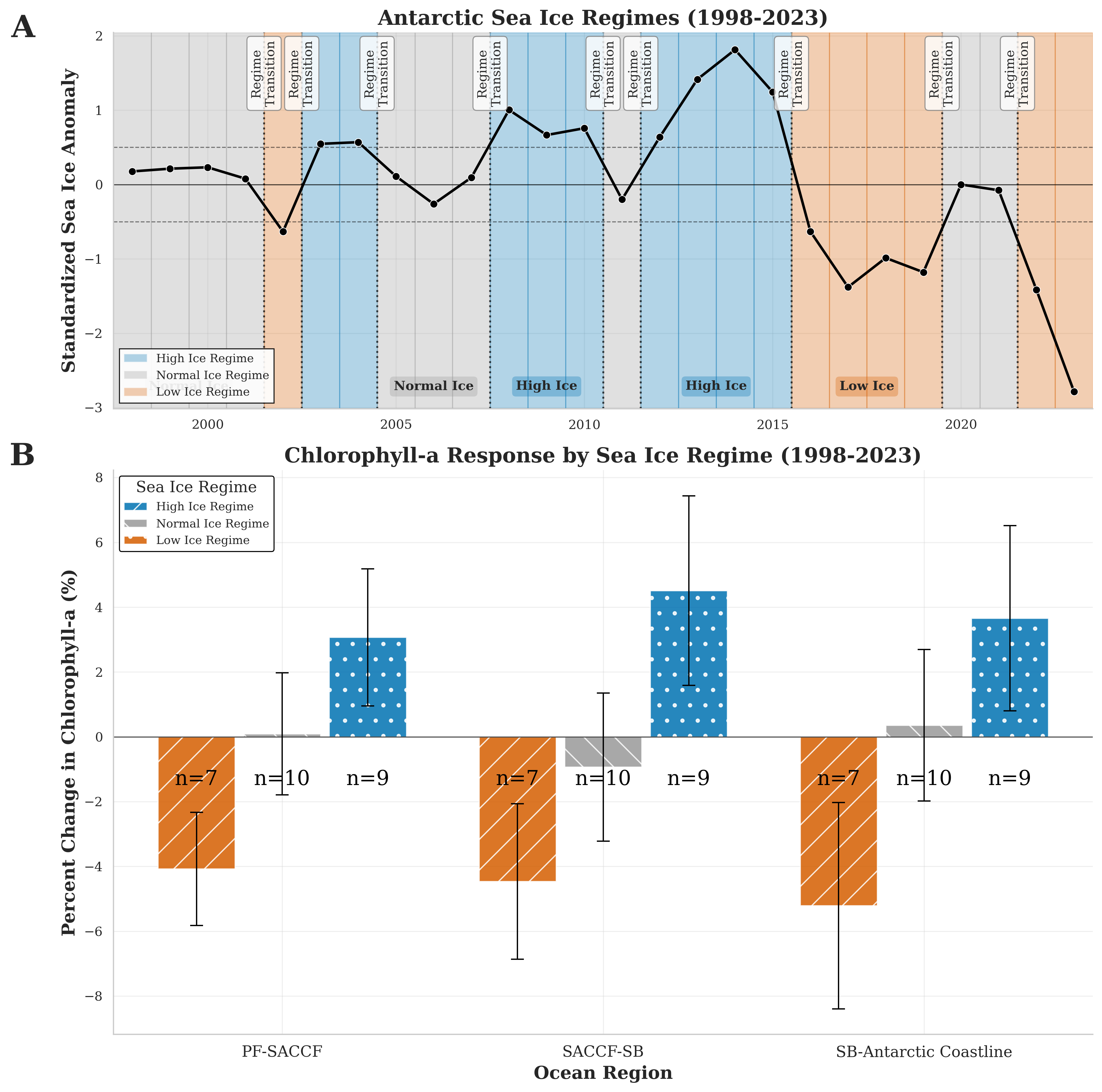
Figure 3.5: Sea ice regimes and regional Chlorophyll-a responses in the Southern Ocean (1998-2023). (A) Standardized sea ice anomalies showing three distinct regimes: High Ice (blue shading), Normal Ice (gray shading), and Low Ice (red shading), defined by thresholds at ±0.5 standard deviations from the climatological mean. (B) Mean percent change in Chlorophyll-a concentration (± standard deviation) across three Southern Ocean zones (PF-SACCF, SACCF-SB, and SB-Antarctic Coastline) during different sea ice regimes. Positive values indicate increased Chlorophyll-a relative to the climatological mean, while negative values indicate decreased Chlorophyll-a. Error bars represent one standard deviation; n values indicate the number of years in each regime. PF = Polar Front; SACCF = Southern Antarctic Circumpolar Current Front; SB = Southern Boundary.
3.5 Conclusion
Our analysis demonstrates a clear statistical association between Antarctic sea-ice extent anomalies and phytoplankton Chl-a anomalies, particularly in the ice-proximal Southern Boundary and SACCF frontal zones. Statistically significant lagged correlations (r ≈ 0.60–0.64, p < 0.01) explain up to 40% of annual Chl-a variability in these regions, while the relationship is weaker north of the SACCF. After2015, reduced sea ice extent coincided with lower mean Chl-a in the southern frontal zones, marking a recent period of reduced mean phytoplankton biomass in near-coastal areas. However, the present analyses do not directly resolve bloom timing, duration, community composition, nutrient supply, grazing, or carbon export. Therefore, interpretations involving bloom phenology or specific mechanisms should be treated as hypotheses requiring dedicated phenological and process-based analyses. Unlike basin-wide studies, our frontal-scale approach shows that sea ice losses may have regionally variable effects on Southern Ocean phytoplankton biomass, with potential implications for carbon cycling and energy transfer to higher trophic levels. While our 26-year record provides valuable insight into recent variability, longer records and in situ observations are needed to distinguish robust long-term change from interannual variability.