4 Deep Learning-Based Reconstruction of Southern Ocean Phytoplankton

This chapter is an edited version of the manuscript submitted to Remote Sensing of Environment.

4.1 Abstract

Southern Ocean plays a crucial role in global climate regulation and carbon cycling; however, long-term phytoplankton dynamics remain poorly understood due to the limited availability of satellite observations. Here, we apply a U-Net–based deep learning framework that integrates satellite and reanalysis data to reconstruct surface Chlorophyll-a concentrations (Chl-a) based on physical predictors across the Southern Ocean (30°S–85°S) from 2003 to 2017. Using a Mean Absolute Error (MAE) loss function, R² between satellite and reconstructed Chl-a reaches up to 0.73 mg m⁻³ and RMSE 0.35 mg m⁻³. The reconstructed Chl-a fields reproduce observed spatial gradients and seasonal bloom cycles, with the highest skill in the Pacific sector. A permutation feature importance analysis identifies sea surface temperature as the strongest statistical predictor (~40%), followed by sea level anomaly and photosynthetically available radiation, suggesting model sensitivity to spatially coherent, dynamic, and light-related variability rather than direct mechanistic attribution. This study presents the first high-resolution, explainable deep learning reconstruction of phytoplankton variability in the Southern Ocean, bridging physical and biological observations to support improved biogeochemical modelling, ecosystem management, and projections of carbon sequestration under climate change.

4.2 Introduction

The Southern Ocean plays a pivotal role in regulating the global climate and carbon cycling; yet its biological dynamics remain among the least understood due to limitations in observational and modelling efforts. Phytoplankton, the microscopic autotrophs at the basis of the oceanic food web, play a central role in regulating Southern Ocean phytoplankton variability, contributing significantly to carbon sequestration and ecosystem dynamics (Deppeler & Davidson, 2017; Hauck et al., 2023). Monitoring phytoplankton biomass, commonly estimated via Chlorophyll-a concentration (Chl-a), is therefore essential for understanding ocean health and climate feedback.

Since 1997, satellite ocean-colour missions have offered valuable insights into seasonal and interannual dynamics of phytoplankton biomass. However, these satellite records are relatively short and insufficient for capturing low-frequency or multi-decadal-scale variability, which is essential for understanding long-term ecological trends and climate impacts (Martinez et al., 2009). To address this limitation, recent research has increasingly adopted machine learning (ML) techniques to reconstruct extended Chl-a time series using physical oceanographic and atmospheric variables derived from satellite and numerical models (Martinez, Brini, et al., 2020; Martinez, Gorgues, et al., 2020; Navarra et al., 2025; E. Pauthenet et al., 2024; Roussillon et al., 2023).

Two core challenges hinder biogeochemical studies in this region: first, the difficulty in projecting long-term nutrient cycling patterns (Buchovecky et al., 2023), and second, identifying the key physical mechanisms that drive phytoplankton variability (Henley et al., 2020). Traditionally, these challenges have been addressed using coupled physical-biogeochemical models at global (Stock et al., 2020) and regional (Doney, 1999). However, these models typically suffer from coarse spatial resolution and rely on empirically derived parameters, which limit their accuracy and generalizability. Moreover, model biases often make it difficult to confidently link observed biological changes to specific physical drivers.

Early ML efforts employed Support Vector Regression (SVR) and Multi-Layer Perceptrons (MLPs) to predict Chl-a from surface drivers such as sea surface temperature (SST), sea level anomaly (SLA), wind stress, and shortwave radiation (Martinez, Brini, et al., 2020; Martinez, Gorgues, et al., 2020). These models successfully captured large-scale spatial patterns and time variability but underestimated trend amplitudes. More recently, multi-mode Convolutional Neural Networks (CNNs) have been introduced to enhance the reconstruction and interpretability of Chl-a variability by learning region-specific patterns (Roussillon et al., 2023). Here we use a U-Net architecture, a deep convolutional encoder–decoder network originally designed for image segmentation (Ronneberger et al., 2015), which excels at pixel-wise reconstruction and spatial feature learning. Unlike prior CNN approaches, U-Net enables hierarchical feature extraction and full-resolution output, making it well-suited to capturing the complex, multiscale physical–biogeochemical interactions characteristic of high-latitude oceans.

This study addresses key limitations in phytoplankton monitoring by applying a U-Net deep learning framework to reconstruct monthly Chl-a fields at 1/4° resolution across the Southern Ocean from 2003 to 2017. The model is trained on satellite and reanalysis data and evaluated across ocean sectors, seasons, and time periods to assess its generalisation capability. To interpret the influence of physical predictos such as SST, SLA, wind speed, photosynthetically available radiation (PAR), and mixed layer depth (MLD), we employ permutation-based explainability tools. We evaluate whether these predictors provide statistically distinguishable information for Chl-a reconstruction and whether model sensitivity varies across Southern Ocean regions. By combining high-resolution reconstruction with explainability analysis, this framework offers robust predictions and insights into the physical-biogeochemical coupling that governs phytoplankton variability. These advances support improved biogeochemical modelling, ecosystem management (e.g., fisheries and protected areas), and climate mitigation strategies through better projections of oceanic carbon sequestration under future warming scenarios.

4.3 Data and Methods

4.3.1 Physical predictors and Chl-a variables

Phytoplankton growth in the upper ocean is primarily governed by light and nutrient availability, both of which are modulated by physical oceanographic processes. To capture these influences, we use a set of physical predictors that represent key bottom-up controls on phytoplankton variability (Table 4.1). These include sea surface temperature (SST), sea level anomaly (SLA), mixed layer depth (MLD), photosynthetically available radiation (PAR), and surface wind speed. The target variable is surface Chl-a derived from merged satellite products.

Table 4.1. Chlorophyll-a and environmental predictors used for satellite‑based training, their ecological relevance, data products, and native spatio‑temporal resolution. Here, chlorophyll‑a concentratuion (Chl‑a) from GlobColour; sea surface temperature (SST) from the Group for High Resolution Sea Surface Temperature (GHRSST); sea level anomaly (SLA) from the Copernicus Marine Environment Monitoring Service (CMEMS; product generated by Collecte Localisation Satellites, CLS); mixed layer depth (MLD) from CMEMS; photosynthetically available radiation (PAR) from the Moderate Resolution Imaging Spectroradiometer (MODIS); and wind speed (WS) from the Cross‑Calibrated Multi‑Platform (CCMP) winds.

Parameter	Relevance to Chl-a variability	Product & Citation	Spatio-temporal resolution
Chlorophyll-a concentration (Chl-a)	Proxy for phytoplankton biomass	GlobColour-CMEMS (CMEMS, 2023a; Garnesson et al., 2019)	Daily, 4 km
Sea Surface Temperature (SST)	Associated with thermal conditions and potential effects on phytoplankton metabolic rates (Lewandowska et al., 2014; Martinez et al., 2009)	GHRSST SST (Good et al., 2020)	Daily, 0.05°
Sea Level Anomaly (SLA)	Reflects thermocline/pycnocline depth and stratification (Wilson & Adamec, 2001)	AVISO CLS (Pujol & Mertz, 2024)	Daily, 0.125°
Mixed Layer Depth (MLD)	Represents upper-ocean mixing depth and and potential light exposure, and mixing (Carranza & Gille, 2015)	ARMOR3D MLD (CMEMS, 2023b)	Monthly, 0.25°
Photosynthetically Available Radiation (PAR)	Controls photosynthetic activity (Sakamoto et al., 2011)	MODIS PAR (Frouin et al., 2003)	Monthly, 4 km
Wind Speed (WS)	Influences surface fluxes, Ekman pumping, and MLD variability (Hopkins et al., 2021)	CCMP Wind (Wentz et al., 2015)	Monthly, 0.25°

All predictors represent gridded Level 4 reanalysis or satellite fields, interpolated onto a monthly 0.25° grid for the period 2003–2017. These datasets provide consistent spatial coverage of the open Southern Ocean while capturing large-scale physical variability relevant to phytoplankton growth.

4.3.2 Data Pre-processing

All datasets were temporally and spatially averaged to a common monthly frequency on a 1/4° grid. The analysis was restricted to Case 1 waters by excluding regions with bathymetry shallower than 200 meters and focused on high southern latitudes between 30°S and 85°S. Despite initial preprocessing, missing values (NaNs) persisted in the datasets, particularly in Chl-a and PAR due to persistent cloud cover in near Antarctic coastal regions. NaNs in Chl-a outputs were retained, as the model can handle missing target values during training. However, since U-Net cannot process NaNs in input predictors, we applied a time-varying land–ocean mask, assigning zero values to land pixels. During training, these masked areas were excluded from loss computation, ensuring model weights were updated solely based on ocean reconstruction errors. Alternative strategies, such as diffusion-based interpolation to smooth inputs over land (Roussillon et al., 2023), were considered but deemed unnecessary here due to their high computational cost and minimal impact on ocean-focused reconstructions.

Given the log-normal distribution of Chl-a, we applied a natural logarithmic transformation to Chl-a prior to modelling. Reconstructions were back-transformed for comparison with satellite observations. As standard in deep learning, all input predictors and log-transformed Chl-a values were normalised by subtracting their mean and dividing by their standard deviation, promoting stable and efficient training.

4.3.3 Neural Network Scheme

4.3.3.1 U-Net

U-Net has been shown to outperform standard fully convolutional networks in image segmentation tasks (Ronneberger et al., 2015). It employs a symmetric encoder-decoder structure. The encoder extracts image features through a series of convolutional and max-pooling layers, enabling the model to capture contextual information from a large receptive field via sequential down-sampling. The decoder then up-samples these feature maps using transposed convolutional layers. Skip connections between corresponding encoder and decoder layers fuse high-level features from the encoder with up-sampled outputs at the same scale, aiding the decoder in recovering fine-grained details for pixel-wise reconstruction.

In this study, we adapted a U-Net as the core deep learning framework, where each monthly input was configured with multiple channels corresponding to the physical predictors (e.g., SST, SLA, wind speed, PAR, and MLD; see Table 4.1), treating the gridded data as image-like inputs. The output is a single-channel map of reconstructed log(Chl-a). This adaptation leverages U-Net's skip connections to preserve fine-scale spatial features, such as regional gradients in the Southern Ocean's heterogeneous environment, outperforming standard CNNs in capturing multiscale patterns from oceanographic data.

The architecture consisted of three down-sampling levels in the encoder and three up-sampling levels in the decoder. Each convolutional block in the encoder employed two 3×3 convolutional layers with reflective padding, batch normalisation, and ReLU activation functions, followed by a 2×2 max-pooling layer for spatial down-sampling. A dropout layer with a rate of 0.5 was applied after the first convolution in each block to reduce overfitting. The number of filters doubled at each encoder level, starting from 64 and increasing to 128, 256, and ultimately reaching 512 filters at the final encoder stage. In the decoder, bilinear upsampling was used to increase spatial resolution, followed by concatenation with corresponding encoder features via skip connections, and two 3×3 convolutional layers with ReLU activations, batch normalization, and dropout. The final output layer employed a 1×1 convolution to generate the reconstructed Chl-a map, utilising a linear activation function to preserve the continuous nature of the output.

While the model operates in the spatial domain, temporal variability is implicitly captured through the sequential monthly training data, enabling the network to generalise across seasons and years. This U-Net application represents one of the first deep-learning reconstructions of phytoplankton dynamics focused exclusively on the Southern Ocean, where physical complexity and data sparsity present unique challenges.

4.3.4 Permutation-based Explainability of the neural network

To evaluate the relative contribution of each predictors to Chl-a reconstructions, we implemented a model-agnostic explainability method based on Permutation Feature Importance (PFI) (Breiman, 2001; Fisher et al., 2019). This technique assesses model sensitivity by randomly shuffling each input variable independently in the test dataset (while keeping others unchanged) and measuring the degradation in predictive performance. A significant drop in performance indicates that the variable is of high importance.

For each predictor, we generated modified inputs and used the trained U-Net to predict Chl-a. We compared these to reference (non-shuffled) reconstructions using scalar metrics (R², RMSE, MAE, regression slope) and spatial metrics (pixel-wise normalised RMSE and correlation maps). Results were visualised via bar charts that summarised percentage contributions to error metrics and spatial maps that highlighted sensitive regions (e.g., shuffling SST might degrade performance most in bloom-prone coastal areas). This PFI approach is particularly suitable for complex models, such as U-Net, where internal parameters offer limited interpretability, providing insights into driver influences without assuming linearity. However, PFI has limitations in this context: it assumes feature independence and may overestimate the importance of correlated variables (e.g., SST and MLD); it is post-hoc and does not provide causal explanations; and results can vary with random shuffles, although we mitigated this by averaging over 10 permutations.

4.3.5 Learning settings

The dataset was split into non-overlapping periods for training and testing: 2003–2010 for training and 2011–2017 for testing. The testing period was capped at 2017 due to potential shifts in sensor behaviour and data inconsistencies post-2017 (E. Pauthenet et al., 2024), as well as to align with stable sensor counts in the GlobColour multi-sensor dataset (CMEMS, 2023a; Gregg et al., 2017), avoiding artifacts from sensor transitions. This choice improves consistency within the training and testing framework, but it also means that independent observational validation is not available for applying the trained model beyond 2017, including periods of rapid post-2016 sea-ice and biogeochemical change. This limitation is revisited in the Discussion and Conclusion.

The model was trained using the Mean Absolute Error (MAE, i.e. L1) loss function, which penalises errors linearly and is robust to outliers common in Chl-a data (e.g., during blooms). Optimisation employed the Adam algorithm (Kingma & Ba, 2014), which is known for its efficiency in training deep neural networks by adaptively adjusting learning rates based on first and second moments of the gradients. Training was conducted over 300 epochs with a fixed learning rate of 0.001, which provided a balance between convergence speed and stability. A dropout rate of 0.5 was applied during training to mitigate overfitting by randomly deactivating half of the neurons in each iteration, thereby improving the model's generalization performance. Hyperparameters, including learning rate, number of epochs, dropout rate, batch size, and network depth, were systematically tuned through sensitivity analyses, with the final configuration selected to minimize validation error while maintaining model robustness (Table 4.2).

To assess robustness to stochastic optimisation and random weight initialisation, model training was repeated ten times using the same architecture and hyperparameter settings. Summary statistics across the ten runs were used where possible, and individual-run results are interpreted as representative diagnostics rather than definitive measures of model skill.

Table 4.2. Final hyperparameter configuration used for U-Net model training and reconstruction of Chl-a. The listed parameters include the learning rate, number of epochs, dropout rate, batch size, and validation split. These values were determined through targeted sensitivity tests focusing on the loss function, batch size, and training duration (epochs), while other parameters were fixed to ensure stability and reproducibility. The chosen setup provided a balance between computational efficiency and model accuracy, enabling consistent convergence across repeated training runs and forming the basis for subsequent reconstructions and future scenario projections.

Hyperparameter	Tested Values	Final Configuration	Rationale
Loss function	MAE, MSE	MAE	Outperformed MSE on skewed Chl-a distribution
Batch size	4, 8	8	Balanced computational efficiency and stability
Epochs	300, 500	300	Ensured convergence without overfitting
Learning rate	– (fixed)	0.001	Standard choice for stable training
Dropout rate	– (fixed)	0.5	Prevented overfitting
Optimizer	– (fixed)	Adam	Efficient adaptive optimizer
Validation split	– (fixed)	0.2	20% of data reserved for validation

4.3.6 Evaluation Framework

To assess the performance of the U-Net model in reconstructing Chl-a, we employed four quantitative metrics: the root-mean-square error (RMSE), mean absolute error (MAE), the coefficient of determination (R²), and the slope of the linear regression. These metrics were calculated by comparing the reconstructed log-transformed Chl-a time series against GlobColour satellite observations.

The RMSE was computed as:

\(RMSE = \sqrt{\frac{\sum\left( \log\left( Chl \right.\ \right) - \log{({Chl}_{Globcolour})}^{2}}{N}}\)

The MAE was calculated as:

\[\ \ \ \ \ \ \ MAE = = \frac{1}{N}\sum_{i = 1}^{N}\left| (logChl) - \left( \log{Chl}_{Globcolour} \right) \right|\]

The coefficient of determination R² was calculated as:

\({\ \ \ \ \ \ \ \ \ \ \ \ \ \ \ \ \ R}^{2} = (\frac{\sum\left( \log\left( Chl \right.\ \right) - {\overline{\log{Chl}}))\ \ (log}{\left( {Chl}_{Globcolour} \right) - \overline{\log\left( C{hl}_{Globcolour} \right)})}}{N*\sigma_{\log{Chl}}*\sigma_{log({Chl}_{Globcolour})}})^{2}\)

where 𝑁 is the number of samples, 𝜎 denotes the standard deviation, and the overbar indicates the temporal mean over the considered period.

To assess spatial variability, maps of correlation and normalised RMSE (NRMSE) were also generated:

\(NRMSE = \frac{\sqrt{\sum(Chl - {{Chl}_{Globcolour})}^{2}}}{\sqrt{\sum({{Chl}_{Globcolour})}^{2}}}\)

4.4 Results

4.4.1 Evaluation of Loss Functions: MAE versus MSE

To determine the most suitable loss function for reconstructing Chl-a variability in the Southern Ocean, two U-Net models were trained using Mean Absolute Error (MAE) and Mean Squared Error (MSE) objectives under identical configurations (300 epochs, learning rate = 0.001, dropout = 0.5, batch size = 8). Both models converged steadily, but their validation behaviour and predictive accuracy differed substantially.

During the test period (2011–2017), the MAE-based model achieved a higher overall performance, with R² = 0.73, RMSE = 0.35, MAE = 0.24, and regression slope = 0.76, compared to R² = 0.69, RMSE = 0.35, MAE = 0.24, and slope = 0.68 for the MSE-based model. Although both loss functions produced comparable absolute errors, the MAE-trained network better reproduced the amplitude and temporal phase of observed Chl-a variability, resulting in improved correspondence with satellite observations across both bloom and non-bloom periods.

Training–validation diagnostics further revealed that the MAE model exhibited markedly greater stability and generalisation capacity. The MAE model showed a mean training–validation gap of 0.023, with an integrated divergence of 6.66 over 300 epochs, compared to 0.062 and 16.53 for the MSE model. This approximately 2.5-fold reduction in cumulative divergence indicates that MAE training is less prone to overfitting. Correspondingly, validation loss trajectories were smoother and displayed smaller epoch-to-epoch fluctuations (Figure 4.1a–b), whereas MSE showed larger oscillations and a broader gap between training and validation curves.

These results reflect the statistical nature of Chl-a data, which exhibit a log-normal, heavy-tailed distribution due to episodic bloom events. The quadratic penalty of MSE overemphasises rare, high-magnitude residuals, causing instability and overfitting in bloom-prone regions. In contrast, MAE penalises errors linearly, providing a more balanced optimisation that captures both baseline and extreme Chl-a variability without being dominated by outliers.

Based on these results, the MAE loss function was adopted for all subsequent analyses. Its robustness to heavy-tailed error distributions and episodic bloom anomalies makes it particularly suitable for reconstructing Southern Ocean Chl-a, where environmental variability is both extreme and spatially heterogeneous.

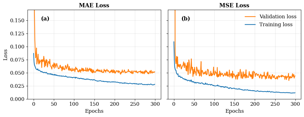
Figure 4.1. Training and validation loss curves for U-Net models using two different loss functions: (a) Mean Absolute Error (MAE) and (b) Mean Squared Error (MSE). Both models were trained for 300 epochs. The blue line represents training loss, and the orange line represents validation loss. MAE shows smoother convergence and a smaller gap between training and validation losses compared to MSE, indicating better generalisation and reduced overfitting.

4.4.2 Statistical Performances

Building on the MAE-optimised U-Net model described in the earlier section, statistical performance was evaluated using scatter plots and spatial maps that compare reconstructed log-transformed Chl-a against GlobColour satellite observations across the Southern Ocean (30°S–85°S). Analyses were conducted for three regional sectors—Pacific, Atlantic, and Indian—and for the full reconstruction period (2003–2017), as well as the training (2003–2010) and the independent testing (2011–2017) phases, to assess spatial consistency and temporal generalisation.

Figure 4.2 shows clear sectoral differences in reconstruction skill. The Pacific sector exhibits the highest statistical agreement, with training metrics of (R² = 0.89, RMSE = 0.11, slope = 0.83) and , testing metrices of (R² = 0.77, RMSE = 0.15, slope = 0.78). , These results indicate that the model reproduces Chl-a variability more consistently in the Pacific sector than in the Atlantic and Indian sectors, although the sectoral framework may mask important variability across Southern Ocean frontal regimes.

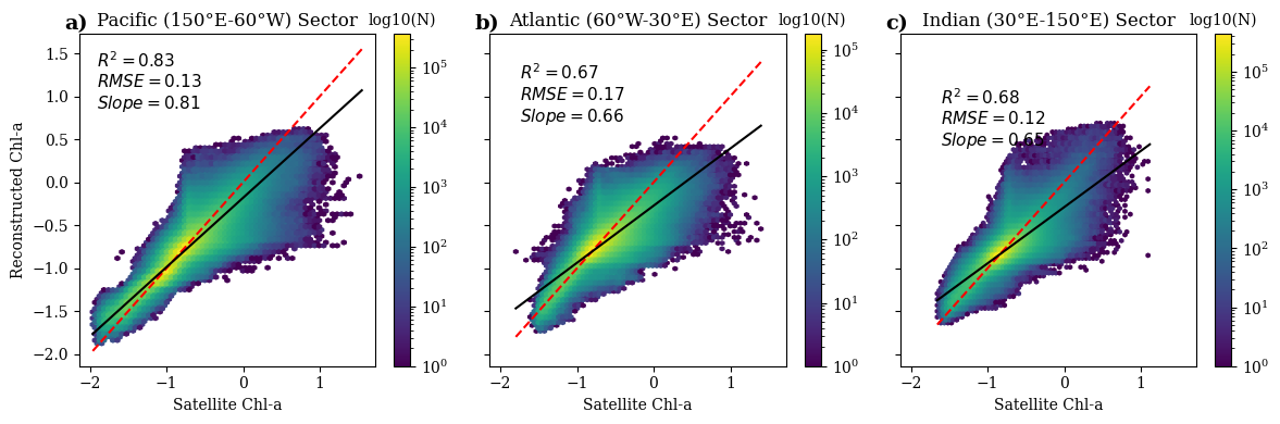
Figure 4.2. Sector-specific scatter plots comparing U-Net reconstructed Chl-a against GlobColour satellite observations across the Southern Ocean during full reconstruction period (2003–2017). Panels show results for the Pacific (150°E–60°W), Atlantic (60°W–30°E), and Indian (30°E–150°E) sectors. Each plot displays log-transformed Chl-a values, with colour density indicating data frequency (log10(N)). Black lines represent linear regression fits, and red dashed lines denote the 1:1 reference. Reported metrics include coefficient of determination (R²), root mean square error (RMSE), and regression slope, highlighting stronger agreement in the Pacific sector and greater deviations in Atlantic and Indian sectors.

By contrast, the Atlantic sector exhibits a larger decrease (R² from 0.80 to 0.53, RMSE from 0.13 to 0.20, and slope from 0.73 to 0.58), while the Indian sector shows a similar degradation (R² from 0.79 to 0.57, RMSE from 0.09 to 0.14, and slope from 0.73 to 0.57) (Figure 4.3). Paired t-tests confirm statistically significant reductions in both R² and slope across sectors (p < 0.05). The regression slopes below unity also indicate that the reconstruction underestimates part of the observed dynamic range, particularly the highest Chl-a values, which should be considered when using the reconstructed fields for downstream interpretation. Across all ten independent U-Net runs, testing-period performance was consistent, with mean R² = 0.695 (range: 0.677–0.719), RMSE = 0.359 (0.343–0.369), MAE = 0.247 (0.236–0.253), and regression slope = 0.725 (0.680–0.782) (Supplementary Table S1). This confirms that the reconstruction skill reported for the representative simulation is broadly consistent with the full ensemble rather than being dependent on a single stochastic training outcome.

Spatial maps of normalized RMSE (NRMSE) and correlation (Figure 4.4) between satellite Chl-a and reconstructed Chl-a complement these findings and illustrate domain-wide performance patterns. NRMSE maps show elevated errors near the Antarctic continent, mostly in coastal and sea-ice-influenced regions during testing, while training values remain lower. Correlation maps display similar gradients, with the highest correlations (r > 0.7) across open-ocean zones between the Subantarctic and Polar Fronts, and weaker relationships (r < 0.5) near Antarctic margins. These results identify where model skill is strongest and weakest without assigning mechanisms in the Results section. The implications of reduced skill in high-latitude and coastal regions are considered in the Discussion.

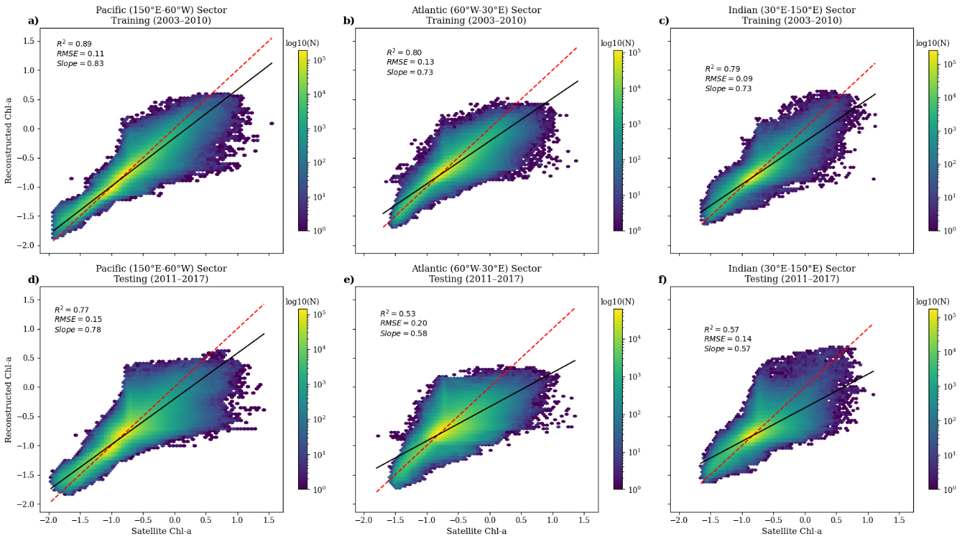
Figure 4.3. Sector-specific scatter plots comparing U-Net reconstructed chlorophyll-a (Chl-a) against CMEMS GlobColour satellite observations across the Southern Ocean. Top row: Training period (2003–2010) for Pacific (150°E–60°W), Atlantic (60°W–30°E), and Indian (30°E–150°E) sectors. Bottom row: Testing period (2011–2017) for the same sectors.

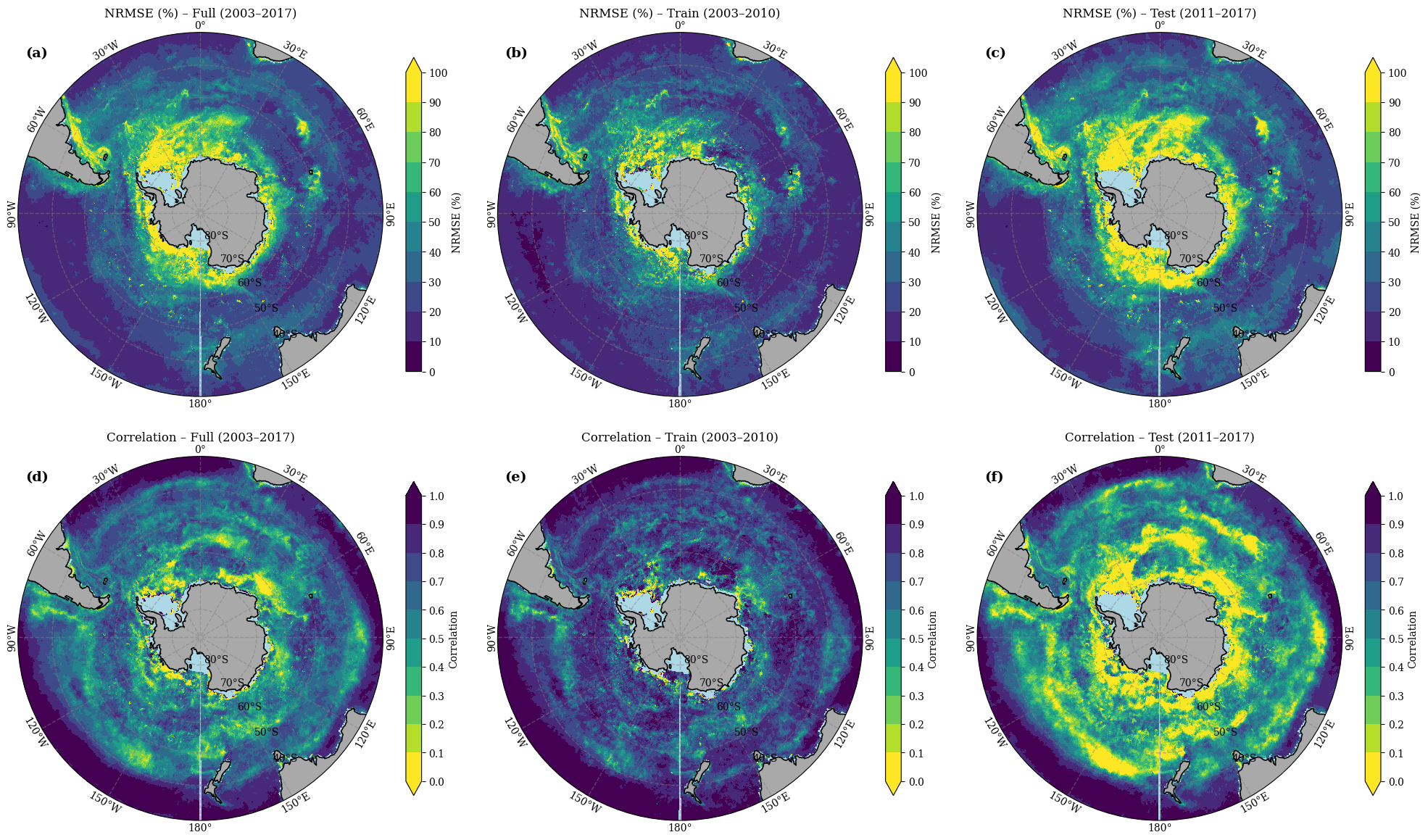
Figure 4.4. Spatial evaluation of U-Net model performance during the training (2003-2010), testing (2011–2017) and full period (203-2017) across the Southern Ocean. Top panel: Normalised Root Mean Square Error (NRMSE, %) between reconstructed and satellite-observed Chl-a, with higher values indicating larger reconstruction errors. Bottom panel: Pixel-wise correlation between reconstructed and satellite-observed Chl-a. Colour scales denote metric ranges for each map.

4.4.3 Spatial and temporal variations in Chl-a

The MAE-optimised U-Net reconstruction reproduces the key spatial and temporal patterns of Chl-a variability across the Southern Ocean (30°S–85°S) during 2003–2017 (Figures 5–6). Mean spatial distributions (Figure 4.5a–b) show that the model captures the large-scale gradients and major high-biomass zones evident in GlobColour satellite observations. Elevated Chl-a concentrations are well represented in the Pacific sector, around the Kerguelen Plateau, and along frontal regions associated with the Subantarctic and Polar Fronts. The spatial difference map (Figure 4.5c; Reconstructed – Satellite) reveals generally strong agreement across open-ocean domains, indicated by near-neutral (white) differences. Systematic underestimations (blue tones) occur primarily in coastal and sea-ice-influenced regions of the Ross and Weddell Seas, while localised overestimations (red patches) appear in portions of the Amundsen Sea and near the Antarctic Peninsula.

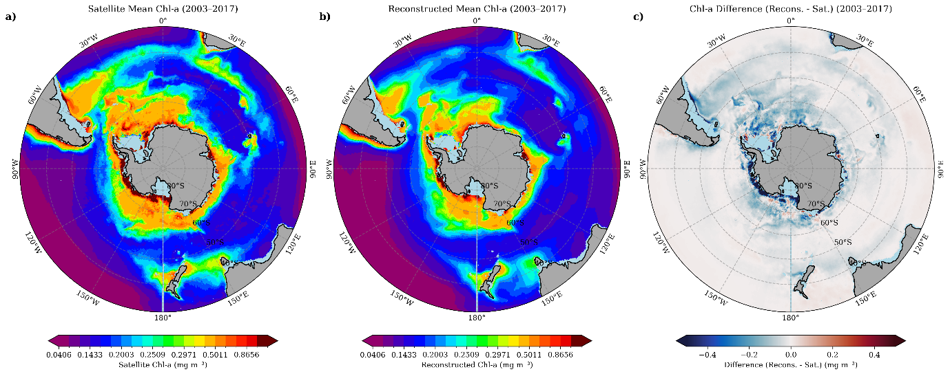
Figure 4.5. Spatial comparison of chlorophyll-a (Chl-a) patterns across the Southern Ocean for the reconstruction period 2003–2017. (a) Satellite-derived mean Chl-a from CMEMS GlobColour observations, (b) U-Net reconstructed mean Chl-a, and (c) difference map (Reconstructed – Satellite). Warmer colors indicate higher Chl-a concentrations, with prominent bloom regions around the Subantarctic and Polar Fronts. The difference map highlights areas of underestimation (blue) near Antarctic coastal zones and overestimation (red) in scattered open-ocean regions.

Temporal analyses further confirm that the model reproduces seasonal and interannual variability of surface Chl-a (Figure 4.6). Median time-series comparisons between reconstructed (red) and satellite-derived (black) Chl-a reveal strong coherence throughout the 2003–2010 training period and sustained alignment into the independent 2011–2017 testing phase. The model captures the timing of the seasonal cycle, including the austral summer bloom peak and winter minima. However, reconstructed values tend to underestimate the magnitude of bloom maxima during the testing years, indicating that the model reproduces phenology more reliably than the full observed amplitude.

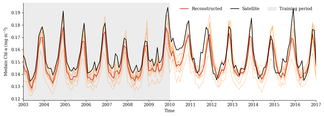
Figure 4.6. Temporal comparison of U-Net reconstructed chlorophyll-a (Chl-a) and CMEMS GlobColour satellite observations across the Southern Ocean from 2003 to 2017.The black line represents the satellite-derived median Chl-a, while the thin orange lines show the ten model runs and their average (thick red line), which indicates the U-Net median prediction. The shaded grey area marks the training period (2003–2010), and the remaining years correspond to the testing period (2011–2017). The model captures seasonal cycles and interannual variability but underestimates bloom peaks, particularly during the testing phase, highlighting challenges in reproducing extreme events.

To complement the Southern Ocean-wide analysis, reconstructed and satellite-derived Chl-a time series were compared within major frontal zones of the Southern Ocean (Supplementary Figure S9). The U-Net reproduces the seasonal cycle and interannual variability across all regions, with correlations ranging from approximately 0.81 to 0.92. The highest agreement is observed between the Polar Front and Southern ACC Front (r ≈ 0.92), while slightly lower skill occurs in coastal Antarctic waters (r ≈ 0.81), where variability is larger and reconstruction errors are more pronounced. Across all frontal zones, the reconstruction captures the timing of bloom development and decline, demonstrating that the framework reproduces phytoplankton variability across contrasting Southern Ocean regimes.

4.4.4 Predictors’ relative importance in Chl-a reconstructions

To better understand the physical–biological relationships learned by the U-Net, we performed a feature importance analysis to evaluate the relative contribution of each environmental driver to Chl-a reconstruction. The results show that SST is the dominant predictor, contributing nearly 40.43% ± 9.63% to the variance across all evaluation metrics (R², RMSE, MAE, and regression slope). This consistent dominance of SST indicates its central role in shaping phytoplankton dynamics in the Southern Ocean. The finding in Figure 4.7 is in agreement with previous studies, such as (Golder & Antoine, 2025), who also identified SST as the primary driver of chlorophyll-a variability. SLA ranks second (22.86% ± 3.29%), reflecting the influence of upper-ocean stratification and pycnocline depth on nutrient availability. PAR follows with 20.26% ± 3.68%, indicating its importance in controlling photosynthetic activity, particularly during seasonal bloom periods. MLD contributes 8.81% ± 5.12%, likely due to its role in modulating light exposure and nutrient entrainment; however, its influence may be dampened by the coarse temporal resolution. Wind speed (WS) contributes the least, at 7.64% ± 4.36%, suggesting a more indirect role through surface mixing and Ekman transport.

Spatially resolved PFI maps (Figure 4.8) reveal heterogeneous patterns of predictor dominance across the Southern Ocean. SST exerts the greatest influence over 47.8 % of the total area, particularly within the Antarctic Circumpolar Current (ACC) and Subantarctic Frontal regions, with notable dominance in the Atlantic sector where strong temperature gradients enhance vertical stratification and nutrient exchange. SLA dominates approximately 22.9 % of the domain, primarily in mesoscale eddy-active regions of the Pacific sector, consistent with its role in vertical nutrient fluxes. Wind speed shows moderate dominance (16.8 %) across the 40°–55°S latitudinal band, particularly in the Indian and Pacific sectors, where enhanced surface stress supports turbulent mixing and modulates bloom development near the sea-ice edge. In contrast, mixed layer depth (9.6 %) displays dominance in more stratified mid-latitude waters, while PAR, though dominant across only 2.7 % of pixels, clusters in highly productive coastal and marginal-ice zones. These localized PAR-driven hotspots suggest strong light control where sea-ice retreat and seasonal irradiance pulses promote short-lived phytoplankton blooms.

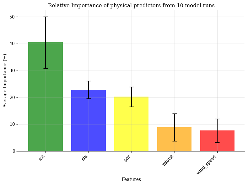
Figure 4.7. Relative contribution of environmental predictors to Chl-a reconstruction, averaged across ten independent U-Net model runs. Bars represent the mean importance (%) of each variable—sea surface temperature (SST), sea level anomaly (SLA), photosynthetically available radiation (PAR), mixed layer depth (MLD), and wind speed (WS)—with error bars indicating inter-run variability. SST consistently emerged as the dominant predictor (~40%), followed by SLA (~25%) and PAR (~20%), while MLD and WS contributed more modestly (~10%), reflecting their secondary roles in shaping phytoplankton dynamics in the Southern Ocean.

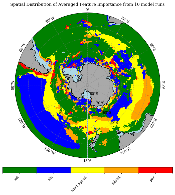
Figure 4.8. Spatial distribution of averaged feature importance for chlorophyll-a (Chl-a) reconstruction across the Southern Ocean, based on permutation feature importance analysis from 10 model runs. Colours represent the dominant predictor in each grid cell: SST (green), SLA (blue), wind speed (yellow), MLD (orange), and PAR (red). SST emerges as the primary driver across most open-ocean regions, while SLA and PAR show localized influence near frontal zones and coastal areas, highlighting regional variability in physical–biological coupling.

4.5 Discussion

To the best of our knowledge, this is the first study to apply a U-Net deep learning framework for reconstructing satellite-derived surface Chl-a in the Antarctic and Southern Ocean, addressing the unique challenges posed by sea-ice, strong seasonality, and limited winter light by integrating satellite and reanalysis data.

The comparative analysis between MAE and MSE loss functions highlights the importance of loss formulation in learning from ocean colour data characterised by strong nonlinearity and skewed error distributions (Pietropolli, 2024). Chl-a in the Southern Ocean exhibits a pronounced log-normal distribution with episodic, high-amplitude blooms (Behrenfeld, 2010; Llido et al., 2005; Montie, 2020). Such distributions challenge conventional optimisation schemes, such as MSE, which amplify large residuals quadratically (Ghosh et al., 2017). Consequently, models trained with MSE tend to overfit extreme bloom events and underperform in low-to-moderate Chl-a regimes (Roussillon et al., 2023; Zhang et al., 2025).

In contrast, MAE applies a linear penalty to deviations, making it inherently more robust to heavy-tailed or heteroscedastic error structures (Alake, 2024; Zhang & Sabuncu, 2018). This robustness explains the smoother convergence, smaller train–validation gaps, and higher generalisation performance observed in this study. The improved regression slope (0.76 versus 0.68) and explained variance (R² = 0.73 vs. 0.69) suggest that MAE helps the network track both the amplitude and phase of Chl-a variability more effectively, thereby avoiding bias toward outlier-driven adjustments. From an oceanographic perspective, the Southern Ocean’s pronounced seasonality, intermittent bloom dynamics, and spatial heterogeneity (influenced by stratification, light availability, sea ice, and mixing) (Ardyna et al., 2017) create a regime where loss functions prioritising stability over extreme sensitivity are advantageous (Terven et al., 2025).

The scatter plots (Figure 4.2-Figure 4.3) reveal clear regional contrasts in the U-Net’s statistical performance. The Pacific sector exhibits the strongest predictive skill, characterised by higher correlations and regression slopes closer to unity. This superior performance likely stems from the strong and predictable physical–biogeochemical coupling driven by basin-scale climate oscillations such as the El Niño–Southern Oscillation (ENSO) and the Pacific Decadal Oscillation (PDO), which regulate SST, SLA, and mixed-layer variability in coherent patterns (Schollaert Uz. et al., 2017). These well-structured relationships allow the network to generalise effectively across bloom and non-bloom regimes. In contrast, the Atlantic and Indian sectors display weaker correlations and greater scatter, reflecting the influence of heterogeneous processes such as intermittent upwelling, subsurface nutrient injections, and coastal variability (Racault et al., 2012; Szeto et al., 2011). Satellite uncertainties due to atmospheric interference and variable optical properties further reduce predictive consistency in these regions. Biological factors also contribute to this spread, as Chl-a variability may reflect photoacclimation or shifts in pigment composition rather than biomass changes (Behrenfeld et al., 2016; Laws & Bannister, 1980). These factors collectively explain the statistically significant decline in R² and slope across non-Pacific sectors (Martinez, Gorgues, et al., 2020).

Spatial patterns of normalised RMSE (NRMSE) and correlation (Figure 4.4) further highlight regional asymmetries in model performance. Regions with higher correlation and lower NRMSE, especially between the Subantarctic and Polar Fronts, correspond to dynamically stable areas where Chl-a variability is strongly constrained by predictable physical drivers (Roussillon et al., 2023). In contrast, elevated errors near the Antarctic shelf and marginal ice zones indicate that the model struggles to capture episodic processes such as melt-induced stratification, iron-limited bloom dynamics, and transient mixing events (Ardyna et al., 2017; Ryan-Keogh et al., 2023).

The absence of explicit ecological predictors, such as grazing pressure or nutrient co-limitation (Moore et al., 2013), further limits model performance in these biologically complex regions. Moreover, unmodeled drivers like atmospheric iron deposition (Cassar et al., 2007; Lancelot et al., 2009) and unresolved mesoscale variability likely amplifies local discrepancies. Collectively, these spatial diagnostics emphasise that model accuracy depends strongly on regional forcing regimes: it excels in dynamically stable frontal zones but weakens in ice-affected, nutrient-limited, and optically complex environments.

The U-Net model’s reconstruction of spatial and temporal Chl-a variability in the Southern Ocean from 2003–2017 effectively captures dominant large-scale patterns while highlighting biases in polar and coastal domains. Mean spatial maps (Figure 4.5a–b) accurately depict elevated Chl-a in the Pacific sector, Kerguelen Plateau, and frontal zones, reflecting enhanced upwelling and nutrient-driven blooms typical of these regions. However, difference maps (Figure 4.5c) show systematic underestimations in coastal areas like the Ross and Weddell Seas, where sea-ice melt and light limitation influence phytoplankton dynamics, often leading to data gaps from cloud cover (Horvat et al., 2022; Mcclish & Bushinsky, 2023; VonBerg et al., 2020). Localised overestimations in the Amundsen Sea and Antarctic Peninsula may arise from the model's sensitivity to unresolved episodic events, consistent with reconstruction biases in polar regions where atmospheric interference complicates satellite-derived inputs (Behera et al., 2020; Ferreira et al., 2020; Kim et al., 2018).

Temporally, the U-Net effectively reproduces seasonal cycles and interannual trends in Chl-a variability (Figure 4.6), with the median time series showing the closest agreement to satellite observations. This robustness reflects the median’s reduced sensitivity to the log-normal outliers typical of bloom events—a behaviour consistent with previous studies reporting improved median-based fits over mean estimates in ocean colour analyses (Etienne Pauthenet et al., 2024). The underestimation of bloom maxima after 2014 likely indicates unmodeled environmental changes, such as ongoing surface warming, mixed-layer shoaling, or sea-ice retreat, as well as potential sensor inconsistencies within the GlobColour dataset (Garcia et al., 2021; Van Oostende et al., 2023). Such temporal degradation aligns with findings from long-term Chl-a reconstructions, where non-stationary ocean dynamics reduce predictive skill during periods unseen by the model (Park et al., 2020). Overall, these results underscore the effectiveness of encoder–decoder architectures, such as U-Net, in capturing spatiotemporal variability and preserving frontal gradients. However, residual coastal and ice-edge biases highlight persistent challenges in representing data-sparse, rapidly changing polar environments.

The U-Net’s feature importance analysis revealed that sea surface temperature (SST) dominated model performance, contributing ~40% ± 9.6% of the total variance. This strong influence aligns with the well-established role of SST as a proxy for upper-ocean stratification, vertical mixing, and nutrient availability (Behrenfeld et al., 2006; Martinez, Brini, et al., 2020). Its broad spatial dominance—covering nearly 48% of the Southern Ocean—further emphasises the thermal control on phytoplankton growth, particularly along the Antarctic Circumpolar Current (ACC) and Subantarctic fronts, where temperature gradients strongly modulate bloom initiation and intensity (Golder & Antoine, 2025). The relatively high importance of SLA underscores the influence of mesoscale and submesoscale variability on nutrient fluxes, particularly within eddy-active regions of the ACC (Ivy Frenger et al., 2018; Swart et al., 2020). This aligns with evidence that dynamic topography modulates subsurface nutrient supply and shapes primary productivity gradients across the ACC fronts. The lower yet regionally significant influence of PAR, concentrated along marginal ice zones, reflects the strong seasonality of light limitation and the biological response to sea-ice retreat (Arrigo et al., 2008; Soppa, 2015). Such localised light control is critical in triggering brief, intense bloom events not fully captured by coarser temporal predictors. Meanwhile, the weaker influence of MLD and wind speed suggests redundancy with SST and SLA, as vertical stability and mixing effects are indirectly encoded in temperature and height anomalies (Tagliabue et al., 2014).

Several predictor-specific limitations are also important. Wind speed represented as a monthly mean is a blunt metric for phytoplankton forcing because biologically important mixing often occurs through episodic high-wind events that deepen the mixed layer, entrain nutrients, and alter light exposure. A future analysis could include storminess metrics, such as the number of days per month exceeding a wind-stress threshold or the variance of daily wind stress. MLD is similarly season-dependent: deep winter mixing can increase the nutrient reservoir available for subsequent blooms, whereas deep summer mixing can suppress growth through light limitation. Combining these opposing seasonal roles into one monthly predictor may cause partial cancellation, so winter and summer MLD should be evaluated separately in future work. Finally, the PAR variable used here represents surface PAR, not underwater light availability; therefore, its regional importance should not be interpreted as a direct sea-ice-modulated underwater light signal without additional attenuation or ice-cover information.

4.6 Conclusions

This study demonstrates the efficacy of a U-Net-based deep learning framework for reconstructing Chl-a fields in the Southern Ocean, overcoming limitations of short satellite records and regional heterogeneity. By integrating multiple physical predictors (SST, SLA, PAR, MLD, and wind speed), the model captures large-scale spatial patterns, seasonal cycles, and interannual variability, with superior statistical performance in the Pacific sector (R² = 0.77 during testing) compared to the Atlantic and Indian sectors. The adoption of MAE loss enhances stability and generalization, particularly for log-normal Chl-a distributions prone to bloom outliers. Permutation-based explainability confirms SST and SLA as the strongest statistical predictors, but these results should be interpreted as model sensitivity rather than direct mechanistic attribution because the predictors are interdependent and several biological controls are not represented.

Despite these advances, challenges persist in high-latitude coastal areas, where sea-ice dynamics, cloud-induced data gaps, episodic mixing, iron limitation and grazing and other unmodelled biological factors contribute to biases. The post-2017 satellite-product caveat also means that there is no fully independent observational ground truth for validating model applications beyond the testing period, which is particularly important given rapid recent changes in Southern Ocean sea ice and associated biogeochemistry. Future extensions should include frontal-zone skill assessments consistent with earlier thesis chapters, ensemble summary statistics across all model runs, storminess metrics, seasonally separated MLD diagnostics, sea-ice and underwater-light information, in situ validation, and climate-projection applications. These additions would strengthen the interpretation of driver dominance and improve the usefulness, of reconstructed fields for understanding Southern Ocean ecosystem change under ongoing warming.